Gravity Inversion#

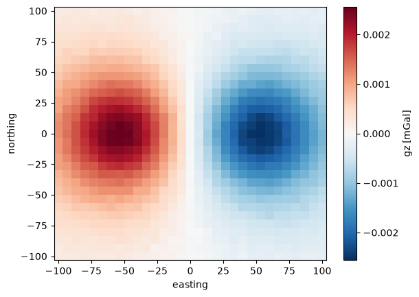
Let’s start this gravity inversion example by generating a synthetic gravity dataset that consists in two prisms with opposite density constrast:

# Plot synthetic data
import matplotlib.pyplot as plt

dataset.gz.plot.pcolormesh(cbar_kwargs={"label": "gz [mGal]"})
plt.show()

Start by defining SimPEG’s gravity simulation for the inversion:

import discretize
import simpeg
from simpeg.potential_fields import gravity

# Define the mesh
h = [(5.0, 40)]
mesh = discretize.TensorMesh(h=[h, h, h], origin="CCN")

# Define gravity survey based on the location of the observation points
easting, northing = dataset.easting, dataset.northing
easting, northing = np.meshgrid(easting, northing)
coordinates = (easting, northing, dataset.upward.values)

locations = np.vstack(tuple(c.ravel() for c in coordinates)).T
receivers = gravity.Point(locations, components="gz")
source = gravity.SourceField(receiver_list=[receivers])
survey = gravity.Survey(source)

# Define SimPEG's gravity simulation
simulation_simpeg = gravity.Simulation3DIntegral(
    mesh, survey=survey, rhoMap=simpeg.maps.IdentityMap(mesh)
)

We need to wrap the simulation to make it compatible with the new inversion framework:

import inversion_ideas as ii

simulation = ii.WrappedSimulation(simulation_simpeg, store_jacobian=True)

Now we can start defining the objective function we want to invert. Let’s start by defining the data misfit using the synthetic data, its errors, and the wrapped simulation:

# Define the data misfit
data = dataset.gz.values.ravel()
uncertainties = dataset.gz_std.values.ravel()
data_misfit = ii.DataMisfit(data, uncertainties, simulation)

Now let’s continue with the regularization:

initial_model = np.zeros(mesh.n_cells)
depth_weights = simpeg.utils.depth_weighting(mesh, 0) ** 2
smallness = ii.Smallness(mesh=mesh, cell_weights=depth_weights)
flatness_x, flatness_y, flatness_z = tuple(
    ii.Flatness(mesh=mesh, direction=direction, cell_weights=depth_weights)
    for direction in ("x", "y", "z")
)
alpha_x, alpha_y, alpha_z = tuple(
    ii.utils.estimate_tradeoff_parameter(smallness, flatness, initial_model)
    for flatness in (flatness_x, flatness_y, flatness_z)
)
model_norm = (
    smallness
    + alpha_x * flatness_x
    + alpha_y * flatness_y
    + alpha_z * flatness_z
).flatten()
model_norm

\[\phi_\text{s} (\mathbf{m}) + 6.635 \, \phi_\text{x} (\mathbf{m}) + 6.621 \, \phi_\text{y} (\mathbf{m}) + 20.218 \, \phi_\text{z} (\mathbf{m})\]

Estimate a trade-off parameter between the data_misfit and the model_norm, and use it as an initial value for the hyperparams.CooledMultiplier:

# Define objective function
beta_0 = 4 * ii.utils.estimate_tradeoff_parameter(data_misfit, model_norm, initial_model)
beta = ii.hyperparams.CooledMultiplier(beta_0, cooling_factor=2)
beta

\[\text{CooledMultiplier}(2.585 \cdot 10^{6})\]

And finally, define the objective function:

phi = data_misfit + beta * model_norm
phi

\[\phi_\text{d} (\mathbf{m}) + \text{CooledMultiplier}(2.585 \cdot 10^{6}) \, [\phi_\text{s} (\mathbf{m}) + 6.635 \, \phi_\text{x} (\mathbf{m}) + 6.621 \, \phi_\text{y} (\mathbf{m}) + 20.218 \, \phi_\text{z} (\mathbf{m})]\]

Build the inversion#

Define a stopping condition: stop the inversion if the \(\chi\) factor falls below 1:

stopping_criterion = ii.conditions.ChiTarget(data_misfit, chi_target=1.0)

Create a dynamic Jacobi preconditioner that will get updated throughout the inversion. Since we’ll need the Inversion to pass it to the minimizer, we’ll pass it to it through the minimizer_kwargs:

preconditioner = ii.JacobiPreconditioner(phi)
minimizer_kwargs = {"preconditioner": preconditioner}

Now we can define the inversion with:

the objective function we want to invert (phi),
the initial model we’ll use to start the inversion process,
a minimize.conjugate_gradient as the minimizer,
the beta.update method as the only directive,
the ChiTarget condition as a stopping criterion,
and the preconditioner inside the minimizer_kwargs dictionary.

inversion = ii.Inversion(
    phi,
    initial_model,
    ii.minimize.conjugate_gradient,
    directives=[beta.update],
    stopping_criterion=stopping_criterion,
    minimizer_kwargs=minimizer_kwargs,
)

And run it!

inverted_model = inversion.run()

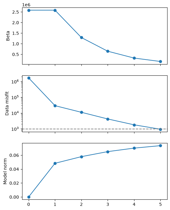
We can access the inversion.log and convert it to a pandas.DataFrame, and also use it to plot convergence curves:

log = inversion.log.to_pandas()
log

	beta	phi_d	phi_m	beta * phi_m	phi	chi
iter
0	2.585145e+06	1.667546e+06	0.000000	0.000000	1.667546e+06	1735.219131
1	2.585145e+06	2.899614e+04	0.048352	124997.124329	1.539933e+05	30.172888
2	1.292572e+06	1.103149e+04	0.057869	74799.776763	8.583127e+04	11.479182
3	6.462862e+05	4.166759e+03	0.065094	42069.293002	4.623605e+04	4.335858
4	3.231431e+05	1.772969e+03	0.070118	22658.162433	2.443113e+04	1.844921
5	1.615716e+05	9.318052e+02	0.073670	11902.945813	1.283475e+04	0.969620

fig, axes = plt.subplots(nrows=3, ncols=1, sharex=True, figsize=(6, 8))
axes[0].plot(log.index, log.beta, "o-")
axes[0].set_ylabel("Beta")

axes[1].plot(log.index, log.phi_d, "o-")
axes[1].axhline(data_misfit.n_data, linestyle="--", color="grey")
axes[1].set_ylabel("Data misfit")
axes[1].set_yscale("log")

axes[2].plot(log.index, log.phi_m, "o-")
axes[2].set_ylabel("Model norm")
plt.show()

../../_images/gravity-inversion_13_0.png

Finally, let’s plot the model:

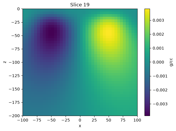
(tmp,) = mesh.plot_slice(inverted_model, normal="Y", slice_loc=0)
plt.colorbar(tmp, label="g/cc")
plt.show()

../../_images/gravity-inversion_14_0.png