Finite Volume Mesh

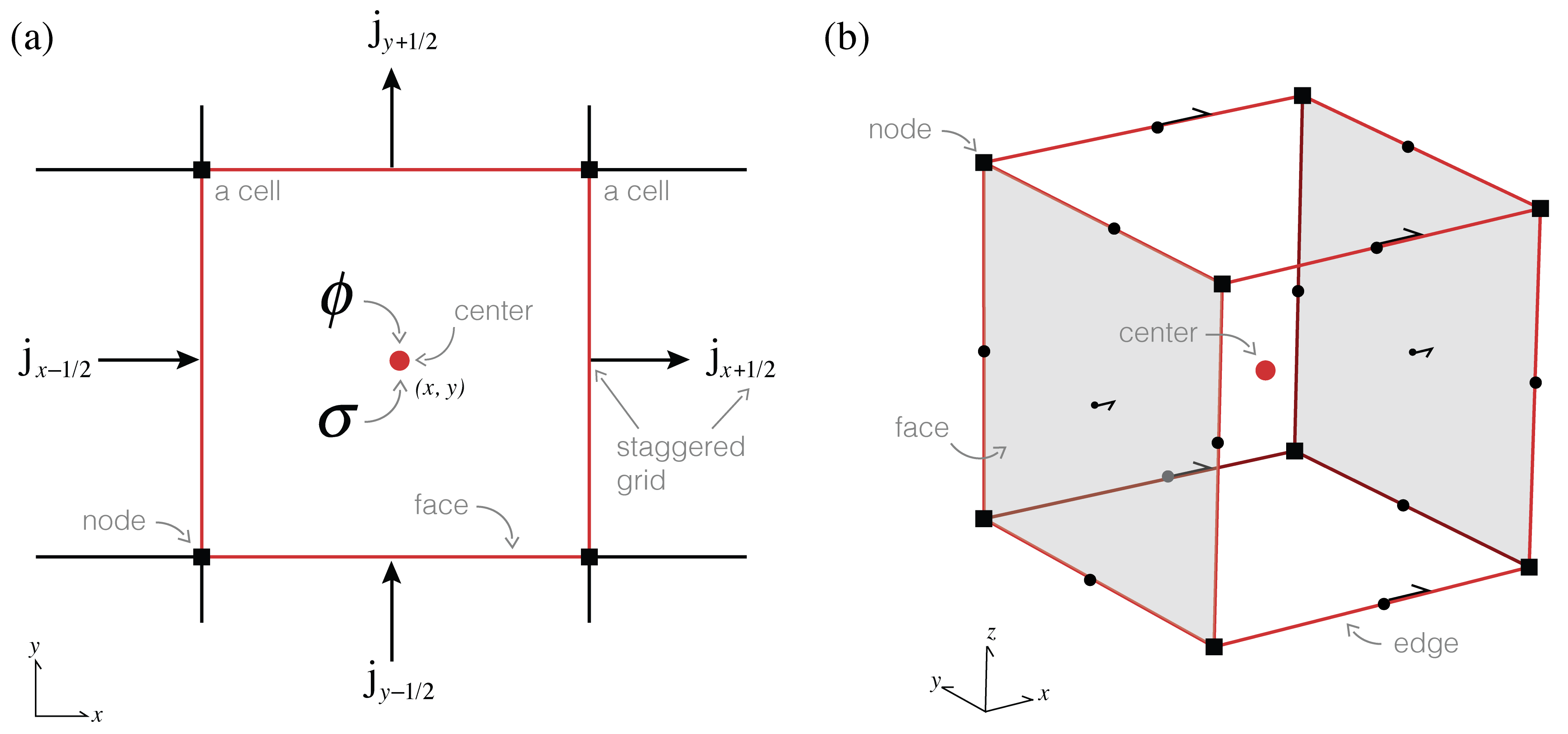
Figure 1:Anatomy of a finite volume cell.

To bring our continuous equations into the computer, we need to discretize the earth and represent it using a finite(!) set of numbers. In this tutorial we will explain the discretization in 2D and generalize to 3D in the notebooks. A 2D (or 3D!) mesh is used to divide up space, and we can represent functions (fields, parameters, etc.) on this mesh at a few discrete places: the nodes, edges, faces, or cell centers. For consistency between 2D and 3D we refer to faces having area and cells having volume, regardless of their dimensionality. Nodes and cell centers naturally hold scalar quantities while edges and faces have implied directionality and therefore naturally describe vectors. The conductivity, $\sigma$ , changes as a function of space, and is likely to have discontinuities (e.g. if we cross a geologic boundary). As such, we will represent the conductivity as a constant over each cell, and discretize it at the center of the cell. The electrical current density, $\vec{j}$ , will be continuous across conductivity interfaces, and therefore, we will represent it on the faces of each cell. Remember that $\vec{j}$ is a vector; the direction of it is implied by the mesh definition (i.e. in $x$ , $y$ or $z$ ), so we can store the array $\bf{j}$ as scalars that live on the face and inherit the face's normal. When $\vec{j}$ is defined on the faces of a cell the potential, $\vec{\phi}$ , will be put on the cell centers (since $\vec{j}$ is related to $\phi$ through spatial derivatives, it allows us to approximate centered derivatives leading to a staggered, second-order discretization).

Implementation¶

%matplotlib inline
import numpy as np
import discretize
import matplotlib.pyplot as plt

Create a Mesh¶

A mesh is used to divide up space, here we will use SimPEG's mesh class to define a simple tensor mesh. By "Tensor Mesh" we mean that the mesh can be completely defined by the tensor products of vectors in each dimension; for a 2D mesh, we require one vector describing the cell widths in the x-direction and another describing the cell widths in the y-direction.

Here, we define and plot a simple 2D mesh using SimPEG's mesh class. The cell centers boundaries are shown in blue, cell centers as red dots and cell faces as green arrows (pointing in the positive x, y - directions). Cell nodes are plotted as blue squares.

# Plot a simple tensor mesh
hx = np.r_[2., 1., 1., 2.]  # cell widths in the x-direction
hy = np.r_[2., 1., 1., 1., 2.]  # cell widths in the y-direction 
mesh2D = discretize.TensorMesh([hx,hy])  # construct a simple SimPEG mesh
mesh2D.plot_grid(nodes=True, faces=True, centers=True);  # plot it!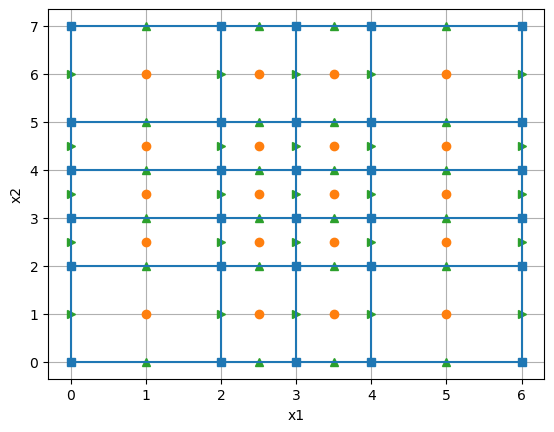

# This can similarly be extended to 3D (this is a simple 2-cell mesh)
hx = np.r_[2.,  2.]  # cell widths in the x-direction
hy = np.r_[2.]  # cell widths in the y-direction 
hz = np.r_[1.]  # cell widths in the z-direction 
mesh3D = discretize.TensorMesh([hx,hy,hz])  # construct a simple SimPEG mesh
mesh3D.plot_grid(nodes=True, faces=True, centers=True);  # plot it!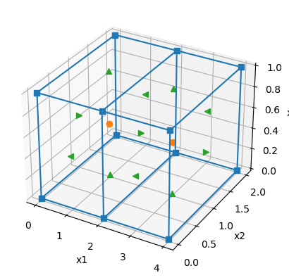

Counting things on the Mesh¶

Once we have defined the vectors necessary for construsting the mesh, it is there are a number of properties that are often useful, including keeping track of the

number of cells: mesh.nC
number of cells in each dimension: mesh.vnC
number of faces: mesh.nF
number of x-faces: mesh.nFx (and in each dimension mesh.vnFx ...) and the list goes on. Check out SimPEG's mesh documentation for more.

# Construct a simple 2D, uniform mesh on a unit square
mesh = discretize.TensorMesh([10, 8])
mesh.plot_grid();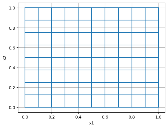

The mesh has 80 cells and 178 faces.

In the $x$ dimension we have 10 cells. This is because our mesh is 10 x 8.

Faces are vectors so the number of faces pointing in the each direction is:

In the $x$ direciton we have 88 faces. (11 x 8)
In the $y$ direciton we have 90 faces. (10 x 9)

Simple properties of the mesh¶

There are a few things that we will need to know about the mesh and each of it's cells, including the

cell volume: mesh.vol,
face area: mesh.area.

For consistency between 2D and 3D we refer to faces having area and cells having volume, regardless of their dimensionality.

# On a uniform mesh, not suprisingly, the cell volumes are all the same
plt.colorbar(mesh.plot_image(mesh.cell_volumes, grid=True)[0])
plt.title('Cell Volumes');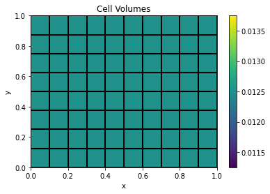

# All cell volumes are defined by the product of the cell widths 
# All cells have the same volume on a uniform, unit cell mesh
assert (np.all(mesh.cell_volumes == 1./mesh.vnC[0] * 1./mesh.vnC[1]))

The cell volume is the product of the cell widths in the $x$ and $y$ dimensions:
0.1 x 0.125 = 0.0125

# Similarly, all x-faces should have the same area, equal to that of the length in the y-direction
assert np.all(mesh.face_areas[:mesh.nFx] == 1.0/mesh.shape_cells[1])  # because our domain is a unit square

# and all y-faces have an "area" equal to the length in the x-dimension
assert np.all(mesh.face_areas[mesh.nFx:] == 1.0/mesh.shape_cells[0])

mesh.plot_grid(faces=True);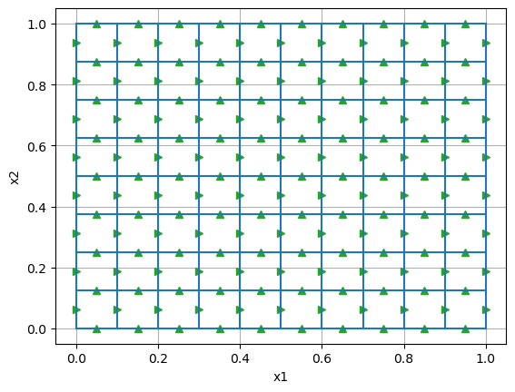

The area of the x-faces is 0.125 and the area of the y-faces is 0.1.

# On a non-uniform tensor mesh, the first mesh we defined, the cell volumes vary

# hx = np.r_[2., 1., 1., 2.]  # cell widths in the x-direction
# hy = np.r_[2., 1., 1., 1., 2.]  # cell widths in the y-direction 
# mesh2D = Mesh.TensorMesh([hx,hy])  # construct a simple SimPEG mesh

plt.colorbar(mesh2D.plot_image(mesh2D.cell_volumes, grid=True)[0])
plt.title('Cell Volumes');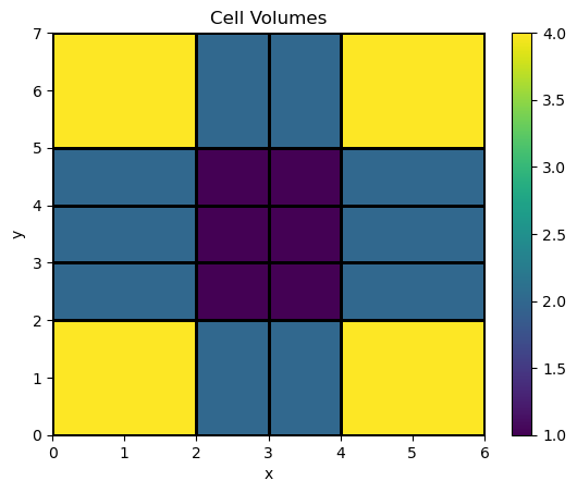

Grids and Putting things on a mesh¶

When storing and working with features of the mesh such as cell volumes, face areas, in a linear algebra sense, it is useful to think of them as vectors... so the way we unwrap is super important.

Most importantly we want some compatibility with Kronecker products as we will see later! This actually leads to us thinking about unwrapping our vectors column first. This column major ordering is inspired by linear algebra conventions which are the standard in Matlab, Fortran, Julia, but sadly not Python. To make your life a bit easier, you can use our MakeVector mkvc function from SimPEG.utils

from SimPEG.utils import mkvc

mesh = discretize.TensorMesh([3,4])

vec = np.arange(mesh.nC)

row_major = vec.reshape(mesh.vnC, order='C')
print('Row major ordering (standard python)')
print(row_major)

col_major = vec.reshape(mesh.vnC, order='F')
print('\nColumn major ordering (what we want!)')
print(col_major)

# mkvc unwraps using column major ordering, so we expect 
assert np.all(mkvc(col_major) == vec)

print('\nWe get back the expected vector using mkvc: {vec}'.format(vec=mkvc(col_major)))

Row major ordering (standard python)
[[ 0  1  2  3]
 [ 4  5  6  7]
 [ 8  9 10 11]]

Column major ordering (what we want!)
[[ 0  3  6  9]
 [ 1  4  7 10]
 [ 2  5  8 11]]

We get back the expected vector using mkvc: [ 0  1  2  3  4  5  6  7  8  9 10 11]

Grids on the Mesh¶

When defining where things are located, we need the spatial locations of where we are discretizing different aspects of the mesh. A SimPEG Mesh has several grids. In particular, here it is handy to look at the

Cell centered grid: mesh.gridCC
x-Face grid: mesh.gridFx
y-Face grid: mesh.gridFy

The cell centered grid is 12 x 2 since we have 12 cells in the mesh and it is 2 dimensions

# The first column is the x-locations, and the second the y-locations

mesh.plot_grid()
plt.plot(mesh.gridCC[:,0], mesh.gridCC[:,1],'ro');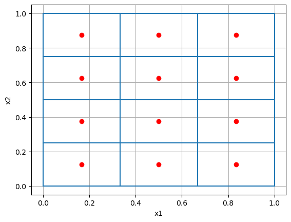

Similarly, the x-Face grid is 16 x 2 since we have 16 x-faces in the mesh and it is 2 dimensions.

mesh.plot_grid()
plt.plot(mesh.gridCC[:,0], mesh.gridCC[:,1],'ro')
plt.plot(mesh.gridFx[:,0], mesh.gridFx[:,1],'g>');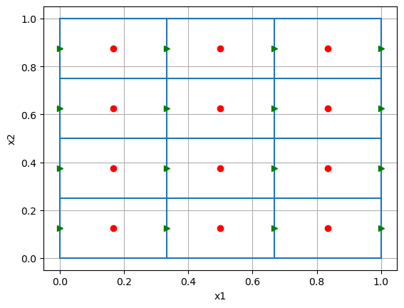

Putting a Model on a Mesh¶

In index.ipynb, we constructed a model of a block in a whole-space, here we revisit it having defined the elements of the mesh we are using.

mesh = discretize.TensorMesh([100, 80])  # setup a mesh on which to solve

# model parameters
sigma_background = 1.  # Conductivity of the background, S/m
sigma_block = 10.  # Conductivity of the block, S/m

# add a block to our model
x_block = np.r_[0.4, 0.6]
y_block = np.r_[0.4, 0.6]

# assign them on the mesh
sigma = sigma_background * np.ones(mesh.nC)  # create a physical property model 

block_indices = ((mesh.gridCC[:,0] >= x_block[0]) & # left boundary 
                 (mesh.gridCC[:,0] <= x_block[1]) & # right boudary
                 (mesh.gridCC[:,1] >= y_block[0]) & # bottom boundary
                 (mesh.gridCC[:,1] <= y_block[1]))  # top boundary

# add the block to the physical property model
sigma[block_indices] = sigma_block

# plot it!
plt.colorbar(mesh.plot_image(sigma)[0])
plt.title('Electrical Conductivity, $\sigma$');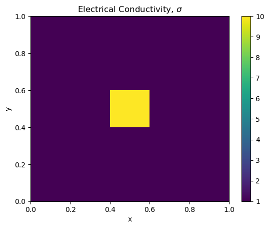

Next up ...¶

In the next notebook, we will work through defining the discrete divergence.