3D Inversion of Gravity Anomaly Data

Author: Devin C. Cowan

Keywords: gravity anomaly, integral formulation, inversion, sparse norm, tensor mesh, tree mesh.

Summary: Here we invert gravity anomaly data to recover a density contrast model. We demonstrate two approaches for recovering a density contrast model:

Weighted least-squares inversion for a tensor mesh
Iteratively re-weighted least-squares (IRLS) inversion for a tree mesh

The weighted least-squares approach is a great introduction to geophysical inversion with SimPEG. One drawback however, is that it recovers smooth structures which may not be representative of the true model. To recover sparse and/or blocky structures, we also demonstrate the iteratively re-weighted least-squares approach. Because this tutorial focusses primarily on inversion-related functionality, we urge the reader to become familiar with functionality explained in the 3D Forward Simulation of Gravity Anomaly Data tutorial before working through this one.

Learning Objectives:

How geophysical inversion is carried out using SimPEG.
How to assign appropriate uncertainties to gravity anomaly data.
How to design a suitable mesh for gravity inversion when using the integral formulation.
How to choose and set parameters for the inversion.
How to define directives that are applied and updated throughout the inversion.
How to applying the sensitivity weighting generally used in 3D gravity inversion.
How to invert data using weighted least-squares and sparse-norm regularization.
How to analyse inversion results.

Although we consider gravity anomaly data in this tutorial, the same approach can be used to invert gravity gradiometry data.

Import Modules¶

Here, we import all of the functionality required to run the notebook for the tutorial exercise. All of the functionality specific to the forward simulation of gravity data are imported from the SimPEG.potential_fields.gravity module. Classes required to define the data misfit, regularization, optimization, etc... are imported from elsewhere within SimPEG. We also import some useful utility functions from SimPEG.utils. To generate the mesh used for the inversion, we use the discretize package.

# SimPEG functionality
from SimPEG.potential_fields import gravity
from SimPEG.utils import plot2Ddata, model_builder, download
from SimPEG import (
    maps,
    data,
    data_misfit,
    inverse_problem,
    regularization,
    optimization,
    directives,
    inversion,
)

# discretize functionality
from discretize import TensorMesh, TreeMesh
from discretize.utils import active_from_xyz

# Common Python functionality
import os
import numpy as np
from scipy.interpolate import griddata
import matplotlib as mpl
import matplotlib.pyplot as plt
import tarfile

mpl.rcParams.update({"font.size": 14})

Load Tutorial Files¶

For most geophysical inversion projects, a reasonable inversion result can be obtained so long as the practitioner has observed data and topography. For this tutorial, the observed data and topography files are provided. Here, we download and import the observed data and topography into the SimPEG framework.

# URL to download from repository assets
data_source = "https://github.com/simpeg/user-tutorials/raw/main/assets/03-gravity/inv_gravity_anomaly_3d_files.tar.gz"

# download the data
downloaded_data = download(data_source, overwrite=True)

# unzip the tarfile
tar = tarfile.open(downloaded_data, "r")
tar.extractall()
tar.close()

# path to the directory containing our data
dir_path = downloaded_data.split(".")[0] + os.path.sep

# files to work with
topo_filename = dir_path + "gravity_topo.txt"
data_filename = dir_path + "gravity_data.obs"

overwriting /home/ssoler/git/user-tutorials/notebooks/03-gravity/inv_gravity_anomaly_3d_files.tar.gz
Downloading https://github.com/simpeg/user-tutorials/raw/main/assets/03-gravity/inv_gravity_anomaly_3d_files.tar.gz

   saved to: /home/ssoler/git/user-tutorials/notebooks/03-gravity/inv_gravity_anomaly_3d_files.tar.gz
Download completed!

For this tutorial, the data are organized within basic XYZ files. However, SimPEG does allow the user to import UBC-GIF formatted gravity data files; see read_grav3d_ubc.

# Load topography (xyz file)
topo_xyz = np.loadtxt(str(topo_filename))

# Load field data (xyz file)
dobs = np.loadtxt(str(data_filename))

Plot Observed Data and Topography¶

Here we plot the synthetic gravity anomaly data and local topography.

# Define receiver locations and observed data
receiver_locations = dobs[:, 0:3]
dobs = dobs[:, -1]

fig = plt.figure(figsize=(9, 5))

ax1 = fig.add_axes([0.05, 0.35, 0.35, 0.6])
plot2Ddata(
    receiver_locations,
    dobs,
    ax=ax1,
    dataloc=True,
    ncontour=40,
    contourOpts={"cmap": "bwr"},
)
ax1.set_title("Gravity Anomaly", pad=15)
ax1.set_xlabel("x (m)")
ax1.set_ylabel("y (m)")

cx1 = fig.add_axes([0.05, 0.18, 0.35, 0.04])
norm1 = mpl.colors.Normalize(vmin=-np.max(np.abs(dobs)), vmax=np.max(np.abs(dobs)))
cbar1 = mpl.colorbar.ColorbarBase(
    cx1, norm=norm1, orientation="horizontal", cmap=mpl.cm.bwr
)
cbar1.set_label("$mGal$", size=16)

ax2 = fig.add_axes([0.55, 0.35, 0.35, 0.6])
plot2Ddata(
    topo_xyz[:, 0:2],
    topo_xyz[:, -1],
    ax=ax2,
    ncontour=50,
    contourOpts={"cmap": "gist_earth"},
)
ax2.set_title("Topography", pad=15)
ax2.set_xlabel("x (m)")
ax2.set_ylabel("y (m)")

cx2 = fig.add_axes([0.55, 0.18, 0.35, 0.04])
norm2 = mpl.colors.Normalize(vmin=np.min(topo_xyz[:, -1]), vmax=np.max(topo_xyz[:, -1]))
cbar2 = mpl.colorbar.ColorbarBase(
    cx2, norm=norm2, orientation="horizontal", cmap=mpl.cm.gist_earth
)
cbar2.set_label("$m$", size=16)

plt.show()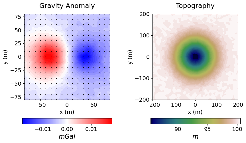

Assign Uncertainties¶

Inversion with SimPEG requires that we define the uncertainties on our data; that is, an estimate of the standard deviation of the noise on our data assuming it is uncorrelated Gaussian with zero mean. An online resource explaining uncertainties and their role in the inversion can be found here.

For gravity anomaly data, a constant floor value is generally applied to all data. We usually avoid assigning percent uncertainties because the inversion would prioritize fitting the background over fitting anomalies. The floor value for the uncertainties may be chosen based on some knowledge of the instrument error, or it may be chosen as some fraction of the largest anomaly value. For this tutorial, the floor uncertainty assigned to all data is 2.5% of the maximum observed gravity anomaly value. For gravity gradiometry data, you may choose to assign a different floor value to each data component.

maximum_anomaly = np.max(np.abs(dobs))
floor_uncertainty = 0.02 * maximum_anomaly
uncertainties = floor_uncertainty * np.ones(np.shape(dobs))
print("Floor uncertainty: {}".format(floor_uncertainty))

Floor uncertainty: 0.00037204

Define the Survey¶

Here, we define the survey geometry. The survey consists of a 160 m x 160 m grid of equally spaced receivers located 5 m above the surface topography. For a more comprehensive description of constructing gravity surveys in SimPEG, see the 3D Forward Simulation of Gravity Anomaly Data tutorial.

# Define the receivers. The data consist of vertical gravity anomaly measurements.
# The set of receivers must be defined as a list.
receiver_list = gravity.receivers.Point(receiver_locations, components="gz")
receiver_list = [receiver_list]

# Define the source field
source_field = gravity.sources.SourceField(receiver_list=receiver_list)

# Define the survey
survey = gravity.survey.Survey(source_field)

Define the Data¶

The SimPEG Data class is required for inversion and connects the observed data, uncertainties and survey geometry.

data_object = data.Data(survey, dobs=dobs, standard_deviation=uncertainties)

Weighted Least-Squares Inversion on a Tensor Mesh¶

Here, we provide a step-by-step best-practices approach for weighted least-squares inversion of gravity anomaly data.

Design a (Tensor) Mesh¶

Meshes are designed using the discretize package. Here, we design a tensor mesh. See the discretize user tutorials to learn more about creating meshes. When designing a mesh for gravity inversion, we must consider the spatial wavelengths of the signals contained within the data. If the data spacing is large and/or the signals present in the data are smooth, larger cells can be used to construct the mesh. If the data spacing is smaller and compact anomalies are observed, smaller cells are needed to characterize the structures responsible. And smaller cells are required when the effects of surface topography are significant.

General rule of thumb: The minimum cell size in each direction is at most 0.5 - 1 times the station spacing. And the thickness of the padding is at least 1 - 2 times the width of the survey region.

# Generate tensor mesh with top at z = 0 m
dh = 5.0  # minimum cell size
hx = [(dh, 5, -1.3), (dh, 40), (dh, 5, 1.3)]  # discretization along x
hy = [(dh, 5, -1.3), (dh, 40), (dh, 5, 1.3)]  # discretization along y
hz = [(dh, 5, -1.3), (dh, 15)]  # discretization along z
tensor_mesh = TensorMesh([hx, hy, hz], "CCN")

# Shift vertically to top same as maximum topography
tensor_mesh.origin += np.r_[0.0, 0.0, topo_xyz[:, -1].max()]

Define the Active Cells¶

Whereas cells below the Earth’s surface contribute towards the simulated gravity anomaly, air cells do not. The set of mesh cells used in the forward simulation are referred to as ‘active cells’. Unused cells (air cells) are ‘inactive cells’. Here, the discretize active_from_xyz utility function is used to find the indices of the active cells using the mesh and surface topography. The output quantity is a bool array.

active_tensor_cells = active_from_xyz(tensor_mesh, topo_xyz)
n_tensor_active = int(active_tensor_cells.sum())

Mapping from the Model to Active Cells¶

In SimPEG, the term ‘model’ is not synonymous with the physical property values defined on the mesh. For whatever model we choose, we must define a mapping from the set of model parameters (a 1D numpy.ndarray) to the active cells in the mesh. Mappings are created using the SimPEG.maps module. For the tutorial exercise, the model is the density contrast values for all active cells. As such, our mapping is an identity mapping, whose dimensions are equal to the number of active cells.

tensor_model_map = maps.IdentityMap(nP=n_tensor_active)

Starting/Reference Models¶

The starting model defines a reasonable starting point for the inversion and does not necessarily represent an initial estimate of the true model. Because the integral formulation used to solve the gravity forward simulation is linear, the optimization problem we must solve is a linear least-squares problem, making the choice in starting model insignificant. It should be noted that the starting model cannot be vector of zeros, otherwise the inversion will be unable to compute a gradient direction at the first iteration. For gravity inversion, the starting model is frequently a constant vector with a very small value.

The reference model is used to include a-prior information. The impact of the reference model on the inversion will be discussed in another tutorial. Assuming the contribution from all background structures has been removed from the gravity anomaly data, and assuming we have not a-priori information, the reference model for basic inversion of gravity data is zero.

Notice that the length of the starting and reference models is equal to the number of active mesh cells!!!

starting_tensor_model = 1e-6 * np.ones(n_tensor_active)
reference_tensor_model = np.zeros_like(starting_tensor_model)

# Map for ignoring inactive cells when plotting
tensor_plotting_map = maps.InjectActiveCells(tensor_mesh, active_tensor_cells, np.nan)

fig = plt.figure(figsize=(7, 3))
ax1 = fig.add_axes([0.1, 0.1, 0.73, 0.8])

norm = mpl.colors.Normalize(vmin=-0.1, vmax=0.1)
tensor_mesh.plot_slice(
    tensor_plotting_map * starting_tensor_model,
    normal="Y",
    ax=ax1,
    ind=int(tensor_mesh.shape_cells[1] / 2),
    grid=True,
    pcolor_opts={"cmap": mpl.cm.RdYlBu_r, "norm": norm},
)
ax1.set_title("Starting Model (slice at y = 0 m)")

ax2 = fig.add_axes([0.85, 0.1, 0.03, 0.8])
cbar = mpl.colorbar.ColorbarBase(
    ax2, norm=norm, orientation="vertical", cmap=mpl.cm.RdYlBu_r
)
cbar.set_label("$g/cm^3$", rotation=270, labelpad=15, size=16)

plt.show()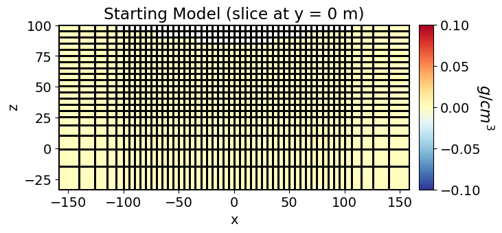

Define the Forward Simulation¶

A simulation object defining the forward problem is required in order to predict data and calculate misfits for recovered models. A comprehensive description of the simulation object for gravity anomaly data was discussed in the 3D Forward Simulation of Gravity Anomaly Data tutorial. Here, we use the 3D integral formulation.

simulation_L2 = gravity.simulation.Simulation3DIntegral(
    survey=survey,
    mesh=tensor_mesh,
    rhoMap=tensor_model_map,
    ind_active=active_tensor_cells,
)

Define the Data Misfit¶

To understand the role of the data misfit in the inversion, please visit this online resource. Here, we use the L2DataMisfit class to define the data misfit. In this case, the data misfit is the L2 norm of the weighted residual between the observed data and the data predicted for a given model. When instantiating the data misfit object within SimPEG, we must assign an appropriate data object and simulation object as properties.

dmis_L2 = data_misfit.L2DataMisfit(data=data_object, simulation=simulation_L2)

Define the Regularization¶

To understand the role of the regularization in the inversion, please visit this online resource. Here, we use the WeightedLeastSquares regularization class to constrain the inversion result. Here, length scales along x, y and z are used to balance the smallness and smoothness terms. And the reference model is only applied to the smallness term; which is redundant for the tutorial example since we have set the reference model to an array of zeros.

reg_L2 = regularization.WeightedLeastSquares(
    tensor_mesh,
    active_cells=active_tensor_cells,
    length_scale_x=1.0,
    length_scale_y=1.0,
    length_scale_z=1.0,
    reference_model=reference_tensor_model,
    reference_model_in_smooth=False,
)

Define the Optimization Algorithm¶

Here, we use the InexactGaussNewton class to solve the optimization problem using inexact Gauss-Newton. Reasonable default values have generally been set for the properties of each optimization class. However, the user may choose to set custom values; e.g. the accuracy tolerance for the conjugate gradient solver or the number of line searches.

opt_L2 = optimization.InexactGaussNewton(
    maxIter=100, maxIterLS=20, maxIterCG=10, tolCG=1e-2
)

Define the Inverse Problem¶

We use the BaseInvProblem class to fully define the inverse problem that is solved at each beta (trade-off parameter) iteration. The inverse problem requires appropriate data misfit, regularization and optimization objects.

inv_prob_L2 = inverse_problem.BaseInvProblem(dmis_L2, reg_L2, opt_L2)

Provide Inversion Directives¶

Directives represent operations that are carried out during the inversion. Here, we apply common directives for weighted least-squares inversion of gravity data and describe their roles. These are:

UpdateSensitivityWeights: Apply sensitivity weighting to counteract the natural tendancy of potential field inversion to cluster recovered structures near the receivers. Because the 3D integral formulation is linear, the sensitivity weighting is independent of the model and does not need to be updated throughout the inversion, so we set every_iteration=False.
UpdatePreconditioner: Apply Jacobi preconditioner when solving optimization problem.
BetaEstimate_ByEig: Compute and set starting trade-off parameter (beta) based on largest eigenvalues.
BetaSchedule: Size reduction of the trade-off parameter at every beta iteration, and the number of Gauss-Newton iterations for each beta.
TargetMisfit: Terminates the inversion when the data misfit equals the target misfit. A chifact=1 terminates the inversion when the data misfit equals the number of data.

The directive objects are organized in a list. Upon starting the inversion or updating the recovered model at each iteration, the inversion will call each directive within the list in order. The order of the directives matters, and SimPEG will throw an error if directives are organized into an improper order. Some directives, like the BetaEstimate_ByEig are only used when starting the inversion. Other directives, like UpdatePreconditionner, are used whenever the model is updated.

sensitivity_weights = directives.UpdateSensitivityWeights(every_iteration=False)
update_jacobi = directives.UpdatePreconditioner(update_every_iteration=True)
starting_beta = directives.BetaEstimate_ByEig(beta0_ratio=10)
beta_schedule = directives.BetaSchedule(coolingFactor=2.0, coolingRate=1)
target_misfit = directives.TargetMisfit(chifact=1.0)

directives_list_L2 = [
    sensitivity_weights,
    update_jacobi,
    starting_beta,
    beta_schedule,
    target_misfit,
]

Define and Run the Inversion¶

We define the inversion using the BaseInversion class. The inversion class must be instantiated with an appropriate inverse problem object and directives list. The run method, along with a starting model, is respondible for running the inversion. The output is a 1D numpy.ndarray containing the recovered model parameters

# Here we combine the inverse problem and the set of directives
inv_L2 = inversion.BaseInversion(inv_prob_L2, directives_list_L2)

# Run inversion
recovered_tensor_model = inv_L2.run(starting_tensor_model)


                    SimPEG.InvProblem is setting bfgsH0 to the inverse of the eval2Deriv.
                    ***Done using the default solver Pardiso and no solver_opts.***

model has any nan: 0
============================ Inexact Gauss Newton ============================
  #     beta     phi_d     phi_m       f      |proj(x-g)-x|  LS    Comment   
-----------------------------------------------------------------------------
x0 has any nan: 0
   0  8.33e+03  5.58e+04  6.08e-07  5.58e+04    2.09e+05      0

   1  4.16e+03  2.22e+04  1.25e+00  2.74e+04    5.00e+04      0

   2  2.08e+03  1.48e+04  2.52e+00  2.01e+04    3.74e+04      0   Skip BFGS

   3  1.04e+03  8.75e+03  4.59e+00  1.35e+04    2.65e+04      0   Skip BFGS

   4  5.21e+02  4.54e+03  7.43e+00  8.40e+03    1.75e+04      0   Skip BFGS

   5  2.60e+02  2.13e+03  1.06e+01  4.90e+03    1.08e+04      0   Skip BFGS

   6  1.30e+02  9.62e+02  1.37e+01  2.75e+03    6.33e+03      0   Skip BFGS

   7  6.51e+01  4.63e+02  1.63e+01  1.53e+03    3.55e+03      0   Skip BFGS

------------------------- STOP! -------------------------
1 : |fc-fOld| = 0.0000e+00 <= tolF*(1+|f0|) = 5.5789e+03
1 : |xc-x_last| = 5.3038e-02 <= tolX*(1+|x0|) = 1.0002e-01
0 : |proj(x-g)-x|    = 3.5490e+03 <= tolG          = 1.0000e-01
0 : |proj(x-g)-x|    = 3.5490e+03 <= 1e3*eps       = 1.0000e-02
0 : maxIter   =     100    <= iter          =      8
------------------------- DONE! -------------------------

Plot the Data Misfit¶

This step is necessary for determining whether the recovered model accurately reproduces observed anomalies. Here, we plot the observed data, predicted data for the recovered model, and the misfit. As we can see, the predicted data fits the background somewhat better than the anomalies. As a result, you may reassign smaller uncertainties in these areas and re-run the inversion in order to better fit the anomalies. We will do this for the iteratively reweighted least-squares inversion.

# Predicted data with final recovered model.
dpred = inv_prob_L2.dpred

# Observed data | Predicted data | Data misfit
data_array = np.c_[dobs, dpred, dobs - dpred]

fig = plt.figure(figsize=(12, 5))
plot_title = ["Observed", "Predicted", "Data Misfit"]
plot_units = ["mGal", "mGal", "mGal"]

ax1 = 3 * [None]
ax2 = 3 * [None]
norm = 3 * [None]
cbar = 3 * [None]
cplot = 3 * [None]
v_lim = [np.max(np.abs(dobs)), np.max(np.abs(dobs)), np.max(np.abs(dobs - dpred))]

for ii in range(0, 3):
    ax1[ii] = fig.add_axes([0.3 * ii + 0.1, 0.2, 0.27, 0.75])
    norm[ii] = mpl.colors.Normalize(vmin=-v_lim[ii], vmax=v_lim[ii])
    cplot[ii] = plot2Ddata(
        receiver_list[0].locations,
        data_array[:, ii],
        ax=ax1[ii],
        ncontour=30,
        contourOpts={"cmap": "bwr", "norm": norm[ii]},
    )
    ax1[ii].set_title(plot_title[ii])
    ax1[ii].set_xlabel("x (m)")
    if ii == 0:
        ax1[ii].set_ylabel("y (m)")
    else:
        ax1[ii].set_yticks([])

    ax2[ii] = fig.add_axes([0.3 * ii + 0.1, 0.05, 0.27, 0.05])
    cbar[ii] = mpl.colorbar.ColorbarBase(
        ax2[ii], norm=norm[ii], orientation="horizontal", cmap=mpl.cm.bwr
    )
    cbar[ii].ax.locator_params(nbins=3)
    cbar[ii].set_label(plot_units[ii], labelpad=5)

plt.show()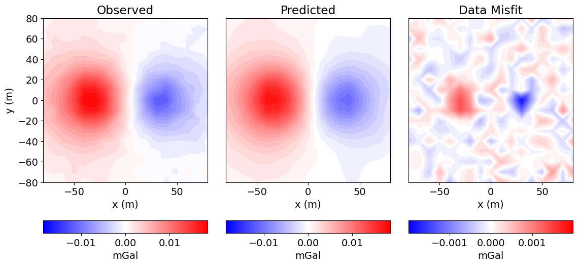

Plot the Recovered Model¶

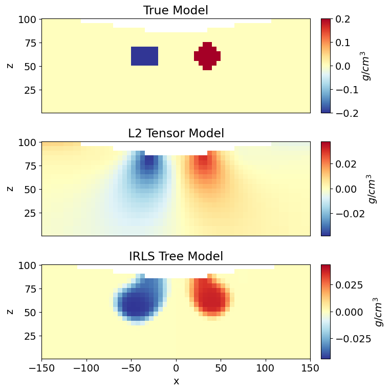
As we can see, weighted least-squares regularization leads to the recovery of smooth models. And even with sensitivity weighting, there is a tendancy for gravity anomaly inversion to place recovered structures near the Earth’s surface.

# Plot Recovered Model
fig = plt.figure(figsize=(7, 3))
ax1 = fig.add_axes([0.1, 0.1, 0.73, 0.8])

norm = mpl.colors.Normalize(
    vmin=np.min(recovered_tensor_model), vmax=np.max(recovered_tensor_model)
)
tensor_mesh.plot_slice(
    tensor_plotting_map * recovered_tensor_model,
    normal="Y",
    ax=ax1,
    ind=int(tensor_mesh.shape_cells[1] / 2),
    grid=False,
    pcolor_opts={"cmap": mpl.cm.RdYlBu_r, "norm": norm},
)
ax1.set_title("Model slice at y = 0 m")

ax2 = fig.add_axes([0.85, 0.1, 0.03, 0.8])
cbar = mpl.colorbar.ColorbarBase(
    ax2, norm=norm, orientation="vertical", cmap=mpl.cm.RdYlBu_r
)
cbar.set_label("$g/cm^3$", rotation=270, labelpad=15, size=16)

plt.show()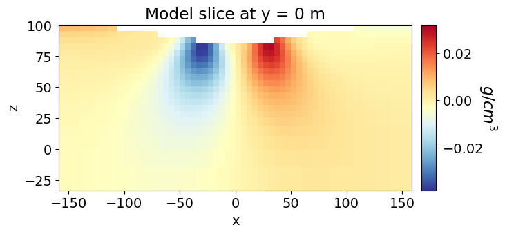

Iteratively Re-weighted Least-Squares (IRLS) Inversion on a Tree Mesh¶

Here, we provide a step-by-step best-practices approach for iteratively IRLS inversion of gravity anomaly data on a tree mesh. Many of the steps are the same as our previous approach. As a result, we will avoid repeating information whenever possible. For the tutorial example, any datum whose normalized data misfit is outside of (-2, 2) will have its uncertainty decreased by a factor of 2.5. This choice was problem dependent!

Reassign the Uncertainties¶

Prior to performing the IRLS inversion, we decrease the uncertainties at the locations we observed the largest data misfits. Here, our goal is to recover a model that better fits the anomalies.

# Compute normalized data misfits
normalized_data_misfits = (dobs - dpred) / uncertainties

# Plot the normalized data misfits
fig = plt.figure(figsize=(6, 3))
ax = fig.add_subplot(111)
ax.plot(np.sort(normalized_data_misfits))
ax.set_title("Normalized Data Misfits (sorted)")
ax.grid()
plt.show(fig)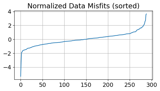

# Generate new uncertainties
new_uncertainties = uncertainties.copy()
new_uncertainties[np.abs(normalized_data_misfits) > 2.0] /= 2.5

# Generate new data object
new_data_object = data.Data(survey, dobs=dobs, standard_deviation=new_uncertainties)

Design a (Tree) Mesh¶

Here, we design a tree mesh. See the discretize user tutorials to learn more about creating tree meshes. The same approach used to construct the tensor mesh used in the weighted least-squares inversion example applies to tree meshes.

dx = 5  # minimum cell width (base tree_mesh cell width) in x
dy = 5  # minimum cell width (base tree_mesh cell width) in y
dz = 5  # minimum cell width (base tree_mesh cell width) in z

x_length = 240.0  # domain width in x
y_length = 240.0  # domain width in y
z_length = 120.0  # domain width in z

# Compute number of base tree_mesh cells required in x and y
nbcx = 2 ** int(np.round(np.log(x_length / dx) / np.log(2.0)))
nbcy = 2 ** int(np.round(np.log(y_length / dy) / np.log(2.0)))
nbcz = 2 ** int(np.round(np.log(z_length / dz) / np.log(2.0)))

# Define the base tree_mesh
hx = [(dx, nbcx)]
hy = [(dy, nbcy)]
hz = [(dz, nbcz)]
tree_mesh = TreeMesh([hx, hy, hz], x0="CCN")

# Shift vertically to top same as maximum topography
tree_mesh.origin += np.r_[0.0, 0.0, topo_xyz[:, -1].max()]

# Refine based on surface topography
tree_mesh.refine_surface(topo_xyz, padding_cells_by_level=[2, 2], finalize=False)

# Refine box based on region of interest
wsb_corner = np.c_[-100, -100, 20]
ent_corner = np.c_[100, 100, 100]
# Note -1 is a flag for smallest cell size
tree_mesh.refine_box(wsb_corner, ent_corner, levels=[-1], finalize=False)

tree_mesh.finalize()

Define the Active Cells¶

active_tree_cells = active_from_xyz(tree_mesh, topo_xyz)
n_tree_active = int(active_tree_cells.sum())

Mapping from Model to Active Cells¶

tree_model_map = maps.IdentityMap(nP=n_tree_active)

Starting and Reference Models¶

starting_tree_model = 1e-6 * np.ones(n_tree_active)
reference_tree_model = np.zeros_like(starting_tree_model)

Define the Forward Simulation¶

simulation_irls = gravity.simulation.Simulation3DIntegral(
    survey=survey, mesh=tree_mesh, rhoMap=tree_model_map, ind_active=active_tree_cells
)

Define Data Misfit¶

dmis_irls = data_misfit.L2DataMisfit(data=new_data_object, simulation=simulation_irls)

Define the Regularization¶

Here, we use the Sparse regularization class to constrain the inversion result using an IRLS approach. Here, the scaling constants that balance the smallness and smoothness terms are set directly. Equal emphasis on smallness and smoothness is generally applied by using the inverse square of the smallest cell dimension. The reference model is only applied to the smallness term; which is redundant for the tutorial example since we have set the reference model to an array of zeros. Here, we apply a 0-norm to the smallness term and a 1-norm to first-order smoothness along the x, y and z directions.

reg_irls = regularization.Sparse(
    tree_mesh,
    active_cells=active_tree_cells,
    alpha_s=dh**-2,
    alpha_x=1,
    alpha_y=1,
    alpha_z=1,
    reference_model=reference_tree_model,
    reference_model_in_smooth=False,
    norms=[0, 1, 1, 1],
)

Define the Optimization Algorithm¶

Here, we use the ProjectedGNCG class to solve the optimization problem using projected Gauss-Newton conjugate gradient. This opimization class allows the user to set upper and lower bounds for the recovered model using the upper and lower properties.

opt_irls = optimization.ProjectedGNCG(
    maxIter=100, lower=-1.0, upper=1.0, maxIterLS=20, maxIterCG=10, tolCG=1e-2
)

Define the Inverse Problem¶

inv_prob_irls = inverse_problem.BaseInvProblem(dmis_irls, reg_irls, opt_irls)

Provide Inversion Directives¶

Here, we create common directives for IRLS inversion of gravity data and describe their roles. In additon to the UpdateSensitivityWeights, UpdatePreconditioner and BetaEstimate_ByEig (described before), inversion with sparse-norms requires the Update_IRLS directive.

You will notice that we don’t use the BetaSchedule and TargetMisfit directives. Here, the beta cooling schedule is set in the Update_IRLS directive using the coolingFactor and coolingRate properties. The target misfit for the L2 portion of the IRLS approach is set with the chifact_start property.

sensitivity_weights_irls = directives.UpdateSensitivityWeights(every_iteration=False)
starting_beta_irls = directives.BetaEstimate_ByEig(beta0_ratio=10)
update_jacobi_irls = directives.UpdatePreconditioner(update_every_iteration=True)
update_irls = directives.Update_IRLS(
    coolingFactor=2,
    coolingRate=1,
    chifact_start=1.0,
    f_min_change=1e-4,
    max_irls_iterations=25,
)

directives_list_irls = [
    update_irls,
    sensitivity_weights_irls,
    starting_beta_irls,
    update_jacobi_irls,
]

Define and Run the Inversion¶

inv_irls = inversion.BaseInversion(inv_prob_irls, directives_list_irls)
recovered_tree_model = inv_irls.run(starting_tree_model)


                    SimPEG.InvProblem is setting bfgsH0 to the inverse of the eval2Deriv.
                    ***Done using the default solver Pardiso and no solver_opts.***

model has any nan: 0
=============================== Projected GNCG ===============================
  #     beta     phi_d     phi_m       f      |proj(x-g)-x|  LS    Comment   
-----------------------------------------------------------------------------
x0 has any nan: 0
   0  5.70e+06  1.17e+05  1.34e-08  1.17e+05    1.99e+02      0

   1  2.85e+06  9.77e+04  1.51e-03  1.02e+05    1.98e+02      0

   2  1.42e+06  8.59e+04  4.57e-03  9.24e+04    1.97e+02      0   Skip BFGS

   3  7.12e+05  7.06e+04  1.24e-02  7.94e+04    1.97e+02      0   Skip BFGS

   4  3.56e+05  5.33e+04  3.00e-02  6.40e+04    1.96e+02      0   Skip BFGS

   5  1.78e+05  3.62e+04  6.44e-02  4.77e+04    1.94e+02      0   Skip BFGS

   6  8.91e+04  2.15e+04  1.23e-01  3.25e+04    1.93e+02      0   Skip BFGS

   7  4.45e+04  1.10e+04  2.06e-01  2.02e+04    1.92e+02      0   Skip BFGS

   8  2.23e+04  4.98e+03  3.00e-01  1.17e+04    1.88e+02      0   Skip BFGS

   9  1.11e+04  2.10e+03  3.89e-01  6.43e+03    1.80e+02      0   Skip BFGS

  10  5.57e+03  9.10e+02  4.62e-01  3.48e+03    1.68e+02      0   Skip BFGS

  11  2.78e+03  4.44e+02  5.19e-01  1.89e+03    1.55e+02      0   Skip BFGS

Reached starting chifact with l2-norm regularization: Start IRLS steps...
irls_threshold 0.037786680460797174

  12  1.39e+03  2.53e+02  9.06e-01  1.51e+03    1.22e+02      0   Skip BFGS

  13  2.48e+03  1.85e+02  1.15e+00  3.03e+03    1.80e+02      0

  14  2.03e+03  3.25e+02  1.09e+00  2.54e+03    1.30e+02      0

  15  2.03e+03  2.74e+02  1.18e+00  2.68e+03    1.55e+02      0

  16  2.03e+03  3.05e+02  1.19e+00  2.73e+03    1.51e+02      0

  17  2.03e+03  3.17e+02  1.20e+00  2.75e+03    1.51e+02      0

  18  1.64e+03  3.35e+02  1.17e+00  2.25e+03    1.10e+02      0

  19  1.64e+03  3.08e+02  1.15e+00  2.20e+03    1.48e+02      0

  20  1.35e+03  3.22e+02  1.11e+00  1.82e+03    1.03e+02      0

  21  1.35e+03  3.02e+02  1.06e+00  1.73e+03    1.46e+02      0

  22  1.35e+03  3.10e+02  1.00e+00  1.66e+03    1.47e+02      0

  23  1.12e+03  3.18e+02  9.64e-01  1.40e+03    1.12e+02      0

  24  1.12e+03  3.04e+02  9.29e-01  1.34e+03    1.44e+02      0   Skip BFGS

  25  1.12e+03  3.09e+02  8.81e-01  1.29e+03    1.45e+02      0

  26  1.12e+03  3.13e+02  8.32e-01  1.24e+03    1.44e+02      0

  27  1.12e+03  3.17e+02  7.81e-01  1.19e+03    1.46e+02      0

  28  9.25e+02  3.20e+02  7.55e-01  1.02e+03    8.16e+01      0   Skip BFGS

  29  9.25e+02  3.10e+02  7.11e-01  9.67e+02    1.38e+02      0   Skip BFGS

  30  9.25e+02  3.10e+02  6.62e-01  9.22e+02    1.40e+02      0   Skip BFGS

  31  9.25e+02  3.11e+02  6.32e-01  8.95e+02    1.39e+02      0   Skip BFGS

  32  9.25e+02  3.13e+02  5.76e-01  8.46e+02    1.34e+02      0   Skip BFGS

  33  9.25e+02  3.14e+02  5.30e-01  8.04e+02    1.32e+02      0   Skip BFGS

  34  9.25e+02  3.14e+02  5.10e-01  7.86e+02    1.33e+02      0   Skip BFGS

  35  9.25e+02  3.14e+02  4.77e-01  7.55e+02    1.24e+02      0   Skip BFGS

  36  9.25e+02  3.13e+02  4.43e-01  7.23e+02    1.22e+02      0   Skip BFGS

Reach maximum number of IRLS cycles: 25
------------------------- STOP! -------------------------
1 : |fc-fOld| = 0.0000e+00 <= tolF*(1+|f0|) = 1.1702e+04
1 : |xc-x_last| = 4.6488e-02 <= tolX*(1+|x0|) = 1.0002e-01
0 : |proj(x-g)-x|    = 1.2160e+02 <= tolG          = 1.0000e-01
0 : |proj(x-g)-x|    = 1.2160e+02 <= 1e3*eps       = 1.0000e-02
0 : maxIter   =     100    <= iter          =     37
------------------------- DONE! -------------------------

Plot the Data Misfit¶

Here we plot the observed data, predicted and misfit for the IRLS inversion. As we can see from the misfit map, the observed data is now fit equally at all locations.

# Predicted data with final recovered model.
dpred_new = inv_prob_irls.dpred

# Observed data | Predicted data | Data misfit
data_array = np.c_[dobs, dpred_new, dobs - dpred_new]

fig = plt.figure(figsize=(12, 5))
plot_title = ["Observed", "Predicted", "Data Misfit"]
plot_units = ["mGal", "mGal", "mGal"]

ax1 = 3 * [None]
ax2 = 3 * [None]
norm = 3 * [None]
cbar = 3 * [None]
cplot = 3 * [None]
v_lim = [np.max(np.abs(dobs)), np.max(np.abs(dobs)), np.max(np.abs(dobs - dpred_new))]

for ii in range(0, 3):
    ax1[ii] = fig.add_axes([0.3 * ii + 0.1, 0.2, 0.27, 0.75])
    norm[ii] = mpl.colors.Normalize(vmin=-v_lim[ii], vmax=v_lim[ii])
    cplot[ii] = plot2Ddata(
        receiver_list[0].locations,
        data_array[:, ii],
        ax=ax1[ii],
        ncontour=30,
        contourOpts={"cmap": "bwr", "norm": norm[ii]},
    )
    ax1[ii].set_title(plot_title[ii])
    ax1[ii].set_xlabel("x (m)")
    if ii == 0:
        ax1[ii].set_ylabel("y (m)")
    else:
        ax1[ii].set_yticks([])

    ax2[ii] = fig.add_axes([0.3 * ii + 0.1, 0.05, 0.27, 0.05])
    cbar[ii] = mpl.colorbar.ColorbarBase(
        ax2[ii], norm=norm[ii], orientation="horizontal", cmap=mpl.cm.bwr
    )
    cbar[ii].ax.locator_params(nbins=3)
    cbar[ii].set_label(plot_units[ii], labelpad=5)

plt.show()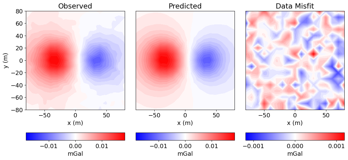

Plot True, L2 and IRLS Models¶

Here, we compare the models recovered from weighted least-squares and iteratively re-weighted least-squares inversion to the true model.

# Recreate True Model on a Tensor Mesh
background_density = 0.0
block_density = -0.2
sphere_density = 0.2

true_model = background_density * np.ones(n_tensor_active)

ind_block = model_builder.get_indices_block(
    [-50, -15, 50], [-20, 15, 70], tensor_mesh.cell_centers[active_tensor_cells]
)
true_model[ind_block] = block_density

ind_sphere = model_builder.get_indices_sphere(
    np.r_[35.0, 0.0, 60.0], 14.0, tensor_mesh.cell_centers[active_tensor_cells]
)
true_model[ind_sphere] = sphere_density

# Plot all models
mesh_list = [tensor_mesh, tensor_mesh, tree_mesh]
ind_list = [active_tensor_cells, active_tensor_cells, active_tree_cells]
model_list = [true_model, recovered_tensor_model, recovered_tree_model]
title_list = ["True Model", "L2 Tensor Model", "IRLS Tree Model"]
cplot = 3 * [None]
cbar = 3 * [None]
norm = 3 * [None]

fig = plt.figure(figsize=(7, 8))
ax1 = [fig.add_axes([0.1, 0.7 - 0.3 * ii, 0.75, 0.23]) for ii in range(0, 3)]
ax2 = [fig.add_axes([0.88, 0.7 - 0.3 * ii, 0.025, 0.23]) for ii in range(0, 3)]

for ii, mesh in enumerate(mesh_list):
    plotting_map = maps.InjectActiveCells(mesh, ind_list[ii], np.nan)
    max_abs = np.max(np.abs(model_list[ii]))
    norm[ii] = mpl.colors.Normalize(vmin=-max_abs, vmax=max_abs)

    cplot[ii] = mesh.plot_slice(
        plotting_map * model_list[ii],
        normal="Y",
        ax=ax1[ii],
        ind=int(mesh.shape_cells[1] / 2),
        grid=False,
        pcolor_opts={"cmap": mpl.cm.RdYlBu_r, "norm": norm[ii]},
    )
    ax1[ii].set_xlim([-150, 150])
    ax1[ii].set_ylim([topo_xyz[:, -1].max() - 100, topo_xyz[:, -1].max()])
    if ii < 2:
        ax1[ii].set_xlabel("")
        ax1[ii].set_xticks([])
    ax1[ii].set_title(title_list[ii])

    cbar[ii] = mpl.colorbar.ColorbarBase(
        ax2[ii], norm=norm[ii], orientation="vertical", cmap=mpl.cm.RdYlBu_r
    )
    cbar[ii].set_label("$g/cm^3$", labelpad=0)

SimPEG User Tutorials

3D Forward Simulation of Gravity Gradiometry Data

SimPEG User Tutorials

Magnetics