Reproduce: SimPEG OcTree

Inverting Pole-Dipole DC Resistivity Data over a Conductive and a Resistive Block

Here, we invert pole-dipole DC resistivity data collected over a conductive and a resistive block. We invert for a conductivity model using a least-squares inversion approach.

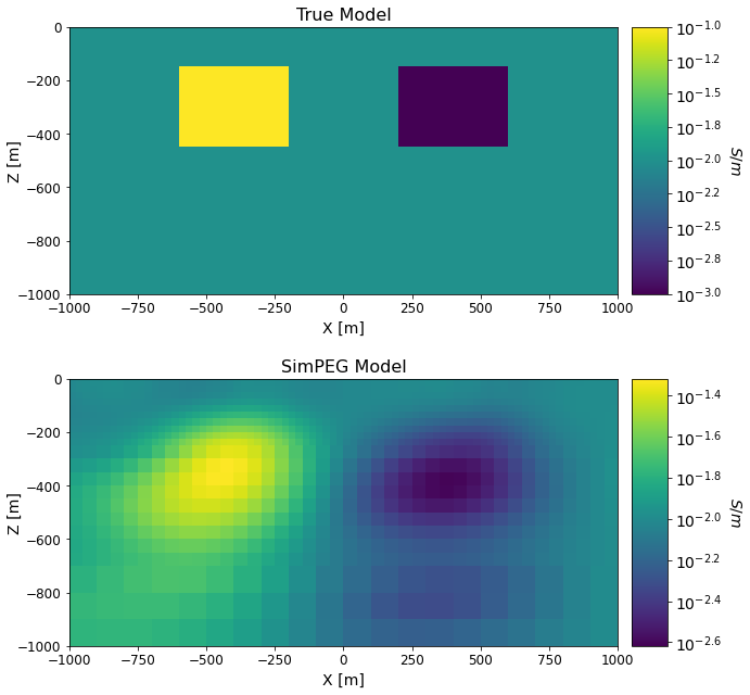
For the true model, the background conductivity \(\sigma_0\) = 0.01 S/m. The conductor has a conductivity of \(\sigma_c\) = 0.1 S/m and the resistor has a conductivity of \(\sigma_r\) = 0.001 S/m. Both blocks are oriented along the Northing direction and have x, y and z dimensions of 400 m, 1600 m and 320 m. Both blocks are buried at a depth of 160 m.

The data being inverted were generated using the SimPEG OcTree code. Synthetic DC voltage data were simulated with a pole-dipole configuration. The survey consisted of 9 West-East survey lines, each with a length of 2000 m. The line spacing was 250 m and the electrode spacing was 100 m. Gaussian noise with a standard deviation of 1e-6 V + 5% the absolute value were added to each datum. Uncertainties of 1e-6 V + 5% were assigned to the data for inversion.

SimPEG Package Details

Link to the docstrings for the simulation class The docstrings will have a citation and show the integral equation.

Running the Inversion

We begin by importing all necessary Python packages for running the notebook.

Show code cell source Hide code cell source

from SimPEG.electromagnetics.static import resistivity as dc
from SimPEG.electromagnetics.static.utils.static_utils import (
    plot_pseudosection,
    plot_3d_pseudosection,
    apparent_resistivity,
    apparent_resistivity_from_voltage,
    convert_survey_3d_to_2d_lines
)
from SimPEG.utils.io_utils import read_dcipoctree_ubc, write_dcipoctree_ubc
from SimPEG import maps, data, data_misfit, regularization, optimization, inverse_problem, inversion, directives
from discretize import TreeMesh
import matplotlib as mpl
import matplotlib.pyplot as plt
import plotly
import numpy as np

try:
    from pymatsolver import Pardiso as Solver
except ImportError:
    from SimPEG import SolverLU as Solver

mpl.rcParams.update({"font.size": 14})
write_output = True

A compressed folder containing the assets required to run the notebook is then downloaded. This includes the mesh, true model, and observed data files.

Show code cell source Hide code cell source

# Import the .tar file

Extracted files are then loaded into the SimPEG framework.

Show code cell source Hide code cell source

rootdir = './../../../assets/dcip/block_model_dc_inv_simpeg_octree/'
meshfile = rootdir + 'octree_mesh.txt'
confile = rootdir + 'true_model.con'
dobsfile = rootdir + 'dobs_simpeg.txt'

mesh = TreeMesh.readUBC(meshfile)
true_conductivity_model = TreeMesh.readModelUBC(mesh, confile)
dc_data = read_dcipoctree_ubc(dobsfile, 'volt')

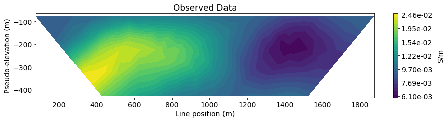
The observed data are measured voltages. And it is voltage data that are inverted. However, here we plot the observed data as apparent conductivities.

Show code cell source Hide code cell source

survey = dc_data.survey
apparent_conductivities = 1/apparent_resistivity_from_voltage(survey, dc_data.dobs, space_type="half space")

plane_points = []
for x in np.arange(-1000, 1100, 500):
    p1, p2, p3 = np.array([-1000.,x,0]), np.array([1000,x,0]), np.array([1000,x,-1000])
    plane_points.append([p1,p2,p3])

scene_camera=dict(
    center=dict(x=-0.1, y=0, z=-0.2), eye=dict(x=1.2, y=-1, z=1.5)
)
scene = dict(
    xaxis=dict(range=[-1000, 1000]), yaxis=dict(range=[-1000, 1000]), zaxis=dict(range=[-500, 0]),
    aspectratio=dict(x=1, y=1, z=0.5)
)

vlim = [apparent_conductivities.min(), apparent_conductivities.max()]
fig = plot_3d_pseudosection(
    dc_data.survey, apparent_conductivities, scale='log', vlim=vlim,
    plane_points=plane_points, plane_distance=10., units='S/m'
)
fig.update_layout(
    title_text="Apparent Conductivities", title_x=0.5, width=600, height=550, scene_camera=scene_camera, scene=scene
)
plotly.io.show(fig)

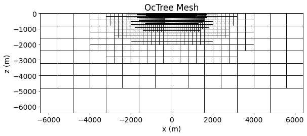
And here we plot the OcTree mesh used in the inversion. Since the topography is flat, all cells are active.

Show code cell source Hide code cell source

ind = int(len(mesh.hy)/2)
fig = plt.figure(figsize=(9, 3.5))
ax1 = fig.add_axes([0.1, 0.12, 0.8, 0.78])
zeros_array = np.zeros(mesh.nC)
mesh.plot_slice(
    zeros_array, ax=ax1, normal='Y', grid=True, ind=ind,
    pcolorOpts={"cmap": "binary"}
)
ax1.set_title("OcTree Mesh")
ax1.set_xlabel("x (m)")
ax1.set_ylabel("z (m)")

Text(0, 0.5, 'z (m)')

Next, we define the mapping from the model space to the mesh and the simulation.

Show code cell source Hide code cell source

sig_map = maps.ExpMap()

simulation = dc.simulation.Simulation3DNodal(
    survey=survey,
    mesh=mesh,
    sigmaMap=sig_map,
    solver=Solver,
    bc_type='Neumann'
)

We now define a starting model for the inversion. We are inverting for the natural log of the conductivity. The starting model is defined based on a known background conductivity of 0.01 S/m.

Show code cell source Hide code cell source

m0 = np.log(1e-2*np.ones(mesh.nC))

Here we define the measure of data misfit, the regularization and the algorithm used to compute the step-direction at each iteration. These are used to define the inverse problem.

Show code cell source Hide code cell source

dmis = data_misfit.L2DataMisfit(data=dc_data, simulation=simulation)

reg_map = maps.IdentityMap(nP=mesh.nC)

reg = regularization.Simple(
    mesh, mapping=reg_map,
    alpha_s=0.1, alpha_x=1., alpha_y=1., alpha_z=1.
)
reg.mrefInSmooth = True

opt = optimization.ProjectedGNCG(
    maxIter=10, maxIterLS=20, maxIterCG=30., tolCG=1e-3
)

inv_prob = inverse_problem.BaseInvProblem(dmis, reg, opt)

Here, we define the directives for the inversion.

Show code cell source Hide code cell source

starting_beta = directives.BetaEstimate_ByEig(beta0_ratio=20.)
beta_schedule = directives.BetaSchedule(coolingFactor=2, coolingRate=2)
save_iteration = directives.SaveOutputEveryIteration(save_txt=False)
target_misfit = directives.TargetMisfit(chifact=1)
sensitivity_weights = directives.UpdateSensitivityWeights(truncation_factor=0.005, threshold=0.)
update_jacobi = directives.UpdatePreconditioner()

directives_list = [
    sensitivity_weights,
    starting_beta,
    beta_schedule,
    save_iteration,
    target_misfit,
    update_jacobi
]

Finally, we define and run the inversion. Using our mapping, we convert the recovered model to the conductivity values defined on the mesh.

Show code cell source Hide code cell source

inv = inversion.BaseInversion(inv_prob, directives_list)
simpeg_model = inv.run(m0)

simpeg_model = sig_map*simpeg_model
dpred = inv_prob.dpred

SimPEG.InvProblem will set Regularization.mref to m0.

        SimPEG.InvProblem is setting bfgsH0 to the inverse of the eval2Deriv.
        ***Done using same Solver and solverOpts as the problem***
model has any nan: 0
=============================== Projected GNCG ===============================
  #     beta     phi_d     phi_m       f      |proj(x-g)-x|  LS    Comment   
-----------------------------------------------------------------------------
x0 has any nan: 0
   0  9.10e+02  3.15e+04  0.00e+00  3.15e+04    1.26e+03      0              
   1  9.10e+02  2.90e+03  4.24e+00  6.76e+03    8.12e+01      0              
   2  4.55e+02  2.50e+03  4.59e+00  4.58e+03    9.64e+01      0   Skip BFGS  
   3  4.55e+02  1.34e+03  6.49e+00  4.30e+03    7.13e+00      0              
   4  2.28e+02  1.37e+03  6.43e+00  2.84e+03    6.66e+01      0              
   5  2.28e+02  7.09e+02  8.44e+00  2.63e+03    3.22e+00      0              
   6  1.14e+02  7.09e+02  8.45e+00  1.67e+03    4.23e+01      0              
------------------------- STOP! -------------------------
1 : |fc-fOld| = 0.0000e+00 <= tolF*(1+|f0|) = 3.1541e+03
1 : |xc-x_last| = 1.5526e+01 <= tolX*(1+|x0|) = 1.8252e+02
0 : |proj(x-g)-x|    = 4.2315e+01 <= tolG          = 1.0000e-01
0 : |proj(x-g)-x|    = 4.2315e+01 <= 1e3*eps       = 1.0000e-02
0 : maxIter   =      10    <= iter          =      7
------------------------- DONE! -------------------------

If desired, we can output the recovered model and the predicted data.

Show code cell source Hide code cell source

if write_output:
    TreeMesh.writeModelUBC(mesh, rootdir+'recovered_model.con', simpeg_model)
    data_dpred = data.Data(survey=dc_data.survey, dobs=dpred)
    write_dcipoctree_ubc(rootdir+'dpred.txt', data_dpred, 'volt', 'dpred')

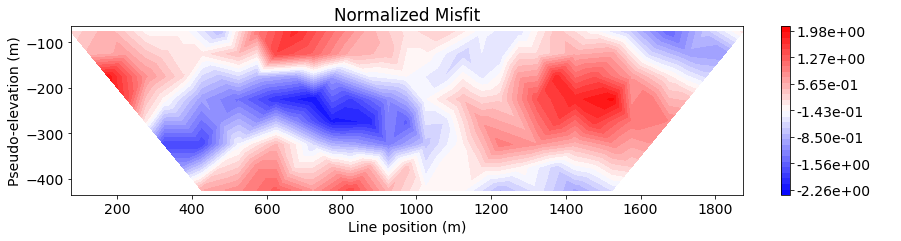
Data Misfit Along a Single Survey Line

Here, we examine the data misfit by plotting a 2D pseudo-section for each survey line. We begin by parsing the 3D survey into a list of 2D surveys.

Show code cell source Hide code cell source

line_id = np.zeros(survey.nD)
northing = np.unique(survey.locations_a[:, 1])

for ii in range(0, len(northing)):
    line_id[survey.locations_a[:, 1] == northing[ii]] = ii

survey_2d_list = convert_survey_3d_to_2d_lines(survey, line_id, 'apparent_chargeability')

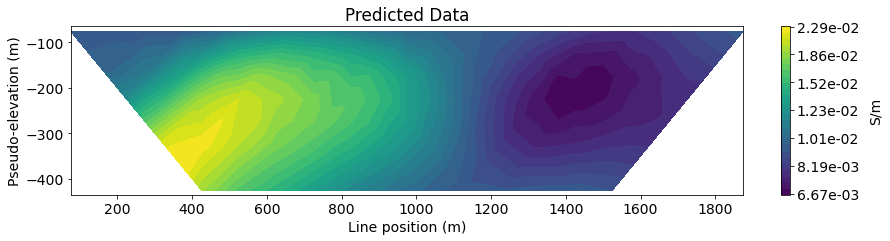
Next, we define the line ID (0-8) for the pole-dipole line we would like to examine. Then plot the observed data, predicted data and normalized misfit in 2D pseudosection.

Show code cell source Hide code cell source

IND = 4
title_str = ['Observed Data', 'Predicted Data', 'Normalized Misfit']
data_list = [
    apparent_conductivities,
    1/apparent_resistivity_from_voltage(survey, dpred, space_type="half space"),
    (dc_data.dobs - dpred) / dc_data.standard_deviation
]
cmap_list = [mpl.cm.viridis, mpl.cm.viridis, mpl.cm.bwr]
label_list = ["S/m", "S/m", " "]
scale_list = ['log', 'log', 'lin']

for ii in range(0, 3):

    fig = plt.figure(figsize=(14, 3))
    ax1 = fig.add_axes([0.1, 0.15, 0.75, 0.78])
    plot_pseudosection(
        survey_2d_list[IND],
        dobs=data_list[ii][line_id==IND],
        plot_type="contourf",
        ax=ax1,
        vlim=vlim,
        scale=scale_list[ii],
        cbar_label=label_list[ii],
        contourf_opts={"levels": 30, "cmap": cmap_list[ii]},
    )
    ax1.set_title(title_str[ii])
    plt.show()

D:\Documents\Repositories\simpeg\SimPEG\electromagnetics\static\utils\static_utils.py:578: UserWarning:

plot_pseudosection unused kwargs: {list(kwargs.keys())}

Comparing True and Recovered Models

Show code cell source Hide code cell source

fig = plt.figure(figsize=(9, 9))
font_size = 14

models_list = [np.log10(true_conductivity_model), np.log10(simpeg_model)]
titles_list = ['True Model', 'SimPEG Model']
ax1 = 2*[None]
cplot = 2*[None]
ax2 = 2*[None]
cbar = 2*[None]

for qq in range(0, 2):
    ax1[qq] = fig.add_axes([0.1, 0.55 - 0.5*qq, 0.78, 0.38])
    
    cplot[qq] = mesh.plot_slice(
        models_list[qq], normal='Y', ind=int(len(mesh.hy)/2), grid=False, ax=ax1[qq]
    )
    cplot[qq][0].set_clim((np.min(models_list[qq]), np.max(models_list[qq])))
    ax1[qq].set_xlim([-1000, 1000])
    ax1[qq].set_ylim([-1000, 0])
    ax1[qq].set_xlabel("X [m]", fontsize=font_size)
    ax1[qq].set_ylabel("Z [m]", fontsize=font_size, labelpad=-5)
    ax1[qq].tick_params(labelsize=font_size - 2)
    ax1[qq].set_title(titles_list[qq], fontsize=font_size + 2)
    
    ax2[qq] = fig.add_axes([0.9, 0.55 - 0.5*qq, 0.05, 0.38])
    norm = mpl.colors.Normalize(vmin=np.min(models_list[qq]), vmax=np.max(models_list[qq]))
    cbar[qq] = mpl.colorbar.ColorbarBase(
        ax2[qq], norm=norm, orientation="vertical", format='$10^{%.1f}$'
    )
    cbar[qq].set_label(
        "$S/m$",
        rotation=270,
        labelpad=20,
        size=font_size,
)

plt.show()