Gravity Inversion: Block in Halfspace (Sparse)#
Geoscientific Problem#
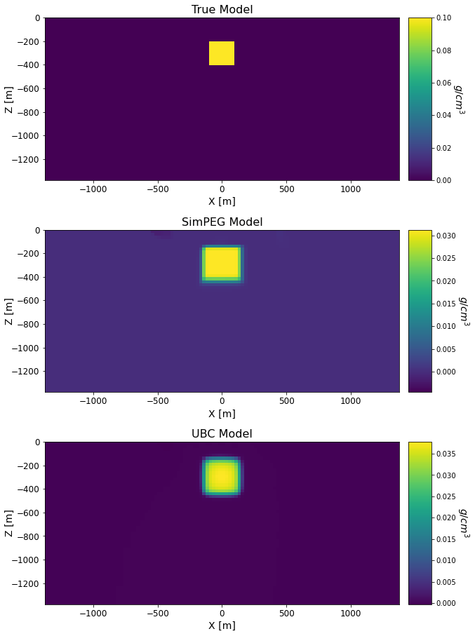
For this code comparison, we inverted gravity anomaly data collected over a block within a homogeneous halfspace. For each coding package, we recovered a compact and blocky model by using an iteratively re-weighted least-squares approach.
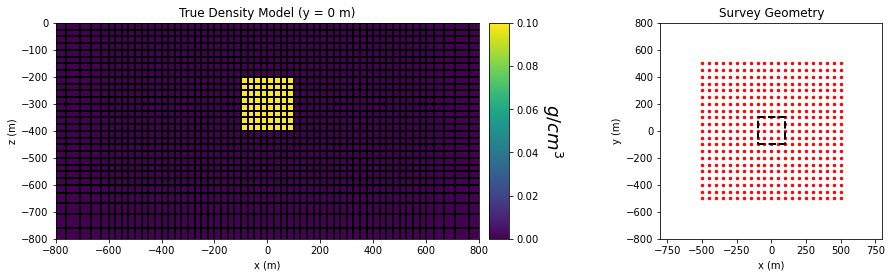
The true model consisted of a block (0.1 \(g/cm^3\)) within a halfspace (0 \(g/cm^3\)). The dimensions of the block in the x, y and z directions were are all 200 m. The block was buried at a depth of 200 m.
The data being inverted were generated using the UBC-GIF GRAV3D v6.0 code. Synthetic gravity data were simulated at a heigh 1 m above the surface within a 1000 m by 1000 m region; the center of which lied directly over the center of the block. Gaussian noise with a standard deviation of 0.002 mGal were added to the synthetic data. Uncertainties of 0.002 mGal were assigned to the data before inverting.
Codes/Formulations Being Compared#
SimPEG 3D Integral Formulation: This approach to solving the forward problem uses the SimPEG.potential_fields.gravity.simulation.Simulation3DIntegral simulation class.
UBC-GIF GRAV3D v6.0: GRAV3D v6.0 is a voxel cell gravity forward modeling and inversion package developed by the UBC Geophysical Inversion Facility. This software is proprietary and can ONLY be acquired through appropriate academic or commerical licenses. The numerical approach of the forward simulation is described in the online manual’s theory section. If you have a valid license, there are instructions for reproducing the results (add link).
Loading Assets Into the SimPEG Framework#
We start by importing any necessary packages for running the notebook.
Show code cell source
from SimPEG.potential_fields import gravity
from SimPEG.utils import plot2Ddata
from SimPEG.utils.io_utils import read_grav3d_ubc
from SimPEG import maps, data_misfit, regularization, optimization, inverse_problem, inversion, directives
from discretize import TensorMesh
import matplotlib as mpl
import matplotlib.pyplot as plt
import numpy as np
Next we download the mesh, true model, recovered model, predicted data and observed data for each coding package/formulation.
Show code cell source
# Download .tar files
For each coding package/formulation, the assets are loaded into the SimPEG framework
Show code cell source
rootdir = './../../../assets/gravity/block_halfspace_gravity_inv_sparse_simpeg/'
mesh_simpeg = TensorMesh.read_UBC(rootdir+'mesh.txt')
true_model_simpeg = TensorMesh.read_model_UBC(mesh_simpeg, rootdir+'true_model.den')
recovered_model_simpeg = TensorMesh.read_model_UBC(mesh_simpeg, rootdir+'recovered_model.den')
dobs_simpeg = read_grav3d_ubc(rootdir+'dobs.grv')
dpred_simpeg = read_grav3d_ubc(rootdir+'dpred.grv')

rootdir = './../../../assets/gravity/block_halfspace_gravity_inv_sparse_grav3d/'
mesh_ubc = TensorMesh.read_UBC(rootdir+'mesh.txt')
true_model_ubc = TensorMesh.read_model_UBC(mesh_simpeg, rootdir+'true_model.den')
recovered_model_ubc = TensorMesh.read_model_UBC(mesh_simpeg, rootdir+'gzinv3d_014.den')
dobs_ubc = read_grav3d_ubc(rootdir+'dobs.grv')
dpred_ubc = read_grav3d_ubc(rootdir+'gzinv3d_014.pre')
True Model and Survey Geometry#
Show code cell source
fig = plt.figure(figsize=(14, 4))

ax11 = fig.add_axes([0.1, 0.15, 0.42, 0.75])
ind = int(mesh_simpeg.shape_cells[1]/2)
mesh_simpeg.plot_slice(
    true_model_simpeg, normal='Y', ind=ind, grid=True, ax=ax11, pcolor_opts={"cmap": "viridis"}
)

ax11.set_xlim([-800, 800])
ax11.set_ylim([-800, 0])
ax11.set_title("True Density Model (y = 0 m)")
ax11.set_xlabel("x (m)")
ax11.set_ylabel("z (m)")

ax12 = fig.add_axes([0.53, 0.15, 0.02, 0.75])
norm = mpl.colors.Normalize(vmin=0, vmax=np.max(true_model_simpeg))
cbar = mpl.colorbar.ColorbarBase(
    ax12, norm=norm, cmap=mpl.cm.viridis, orientation="vertical"
)
cbar.set_label("$g/cm^3$", rotation=270, labelpad=25, size=18)

xyz = dobs_simpeg.survey.receiver_locations
ax21 = fig.add_axes([0.7, 0.15, 0.22, 0.75])
ax21.scatter(xyz[:, 0], xyz[:, 1], 6, 'r')
ax21.plot(100*np.r_[-1, 1, 1, -1, -1], 100*np.r_[-1, -1, 1, 1, -1], 'k--', lw=2)
ax21.set_xlim([-800, 800])
ax21.set_ylim([-800, 800])
ax21.set_title("Survey Geometry")
ax21.set_xlabel("x (m)")
ax21.set_ylabel("y (m)")
Text(0, 0.5, 'y (m)')
Comparing Recovered Models#
Show code cell source
fig = plt.figure(figsize=(9, 14))
font_size = 14

models_list = [true_model_simpeg, recovered_model_simpeg, recovered_model_ubc]
titles_list = ['True Model', 'SimPEG Model', 'UBC Model']
ax1 = 3*[None]
cplot = 3*[None]
ax2 = 3*[None]
cbar = 3*[None]

for qq in range(0, 3):
    ax1[qq] = fig.add_axes([0.1, 0.65 - 0.3*qq, 0.78, 0.23])

    cplot[qq] = mesh_simpeg.plot_slice(
        models_list[qq], normal='Y', ind=int(mesh_simpeg.shape_cells[1]/2), grid=False, ax=ax1[qq]
    )
    cplot[qq][0].set_clim((np.min(models_list[qq]), np.max(models_list[qq])))
    ax1[qq].set_xlabel("X [m]", fontsize=font_size)
    ax1[qq].set_ylabel("Z [m]", fontsize=font_size, labelpad=-5)
    ax1[qq].tick_params(labelsize=font_size - 2)
    ax1[qq].set_title(titles_list[qq], fontsize=font_size + 2)

    ax2[qq] = fig.add_axes([0.9, 0.65 - 0.3*qq, 0.05, 0.23])
    norm = mpl.colors.Normalize(vmin=np.min(models_list[qq]), vmax=np.max(models_list[qq]))
    cbar[qq] = mpl.colorbar.ColorbarBase(
        ax2[qq], norm=norm, orientation="vertical"
    )
    cbar[qq].set_label(
        "$g/cm^3$",
        rotation=270,
        labelpad=20,
        size=font_size,
)

plt.show()
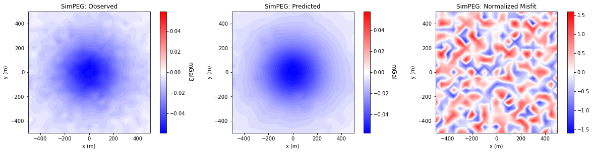
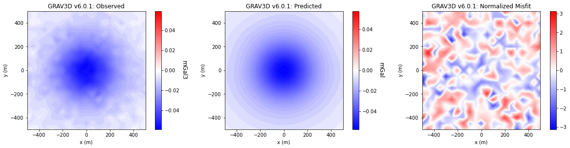
Comparing Misfit Maps#
Show code cell source
data_array = [
    [
        dobs_simpeg.dobs,
        dpred_simpeg.dobs,
        (dobs_simpeg.dobs - dpred_simpeg.dobs) / dobs_simpeg.standard_deviation
    ], [
        dobs_ubc.dobs,
        dpred_ubc.dobs,
        (dobs_ubc.dobs - dpred_ubc.dobs) / dobs_ubc.standard_deviation
    ]
]
code_name = ['SimPEG', 'GRAV3D v6.0.1']

for ii in range(0, len(data_array)):

    fig = plt.figure(figsize=(17, 4))

    plot_title = ["Observed", "Predicted", "Normalized Misfit"]
    plot_units = ["mGal3", "mGal", ""]

    ax1 = 3 * [None]
    ax2 = 3 * [None]
    norm = 3 * [None]
    cbar = 3 * [None]
    cplot = 3 * [None]

    v_lim = [
        np.max(np.abs(data_array[ii][0])),
        np.max(np.abs(data_array[ii][1])),
        np.max(np.abs(data_array[ii][2]))
    ]

    for jj in range(0, 3):

        ax1[jj] = fig.add_axes([0.33 * jj + 0.03, 0.11, 0.25, 0.84])
        cplot[jj] = plot2Ddata(
            xyz,
            data_array[ii][jj],
            ax=ax1[jj],
            ncontour=50,
            clim=(-v_lim[jj], v_lim[jj]),
            contourOpts={"cmap": "bwr"}
        )
        ax1[jj].set_title(code_name[ii] + ': ' + plot_title[jj])
        ax1[jj].set_xlabel("x (m)")
        ax1[jj].set_ylabel("y (m)")

        ax2[jj] = fig.add_axes([0.33 * jj + 0.27, 0.11, 0.01, 0.84])
        norm[jj] = mpl.colors.Normalize(vmin=-v_lim[jj], vmax=v_lim[jj])
        cbar[jj] = mpl.colorbar.ColorbarBase(
            ax2[jj], norm=norm[jj], orientation="vertical", cmap=mpl.cm.bwr
        )
        cbar[jj].set_label(plot_units[jj], rotation=270, labelpad=15, size=12)

    plt.show()