Reproduce: SimPEG#
Inverting Gravity Data Over a Block in a Halfspace: Smoothest Least-Squares#
Here, we invert gravity anomaly data collected over a block within a homogeneous halfspace. We invert for the smoothest model using an unconstrained least-squares inversion approach.
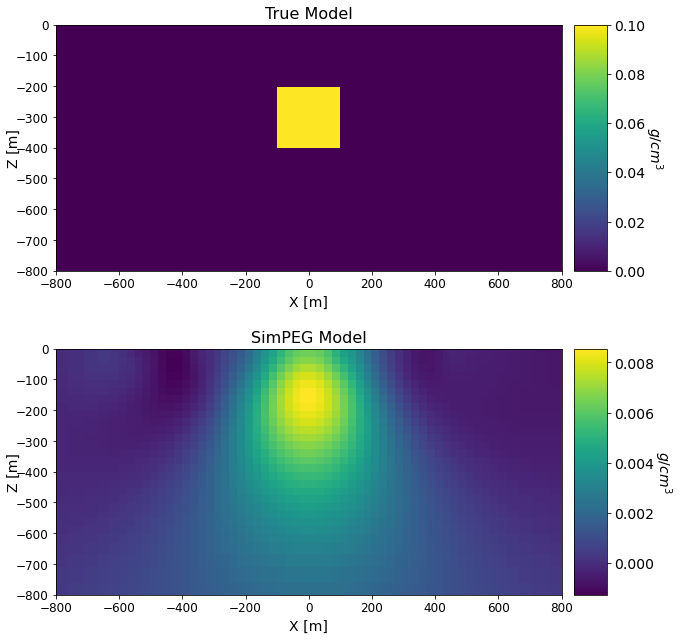
The true model consists of a denser block (0.1 \(g/cm^3\)) within a halfspace (0 \(g/cm^3\)). The dimensions of the block in the x, y and z directions are all 200 m. The block is buried at a depth of 200 m.
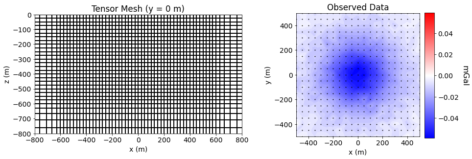
The data being inverted were generated using the UBC-GIF GRAV3D v6.0 code. Synthetic gravity data were simulated at a heigh 1 m above the surface within a 1000 m by 1000 m region; the center of which lied directly over the center of the block. Gaussian noise with a standard deviation of 0.002 mGal were added to the synthetic data. Uncertainties of 0.002 mGal were assigned to the data before inverting.
SimPEG Package Details#
Link to the docstrings for the simulation class. The docstrings will have a citation and show the integral equation.
Reproducing the Inversion Result#
We begin by importing all necessary Python packages for running the notebook.
Show code cell source
from SimPEG import dask
from SimPEG.potential_fields import gravity
from SimPEG.utils import plot2Ddata
from SimPEG.utils.io_utils import read_grav3d_ubc, write_grav3d_ubc
from SimPEG import maps, data, data_misfit, regularization, optimization, inverse_problem, inversion, directives
from discretize import TensorMesh
import matplotlib as mpl
import matplotlib.pyplot as plt
import numpy as np

mpl.rcParams.update({"font.size": 14})
write_output = True
A compressed folder containing the assets required to run the notebook is then downloaded. This includes the mesh, true model, and observed data files.
Show code cell source
# Import the .tar file
Extracted files are then loaded into the SimPEG framework.
Show code cell source
rootdir = './../../../assets/gravity/block_halfspace_gravity_inv_smooth_simpeg/'
meshfile = rootdir + 'mesh.txt'
truemodelfile = rootdir + 'true_model.den'
obsfile = rootdir + 'dobs.grv'
sensitivitydir = './block_halfspace_gravity_inv_smooth_simpeg/'

mesh = TensorMesh.read_UBC(meshfile)
true_model = TensorMesh.read_model_UBC(mesh, truemodelfile)
grav_data = read_grav3d_ubc(obsfile)
We then plot the observed data and the mesh on which we will recover a density contrast model.
Show code cell source
fig = plt.figure(figsize=(14, 4.5))

ax11 = fig.add_axes([0.1, 0.15, 0.42, 0.75])
ind = int(mesh.shape_cells[1]/2)
mesh.plot_slice(
    np.zeros(mesh.nC), normal='Y', ind=ind, ax=ax11,
    pcolor_opts={"cmap": mpl.cm.binary}, grid=True,
)
ax11.set_xlim([-800, 800])
ax11.set_ylim([-800, 0])
ax11.set_title("Tensor Mesh (y = 0 m)")
ax11.set_xlabel("x (m)")
ax11.set_ylabel("z (m)")

ax21 = fig.add_axes([0.63, 0.12, 0.25, 0.8])
xyz = grav_data.survey.receiver_locations
max_val = np.max(np.abs(grav_data.dobs))
plot2Ddata(
    xyz, grav_data.dobs, ax=ax21, dataloc=True, ncontour=50,
    clim=(-max_val, max_val), contourOpts={"cmap": "bwr"}
)
ax21.set_title("Observed Data")
ax21.set_xlabel("x (m)")
ax21.set_ylabel("y (m)")
ax22 = fig.add_axes([0.89, 0.12, 0.02, 0.79])
norm = mpl.colors.Normalize(vmin=-max_val, vmax=max_val)
cbar = mpl.colorbar.ColorbarBase(
    ax22, norm=norm, orientation="vertical", cmap=mpl.cm.bwr
)
cbar.set_label("mGal", rotation=270, labelpad=20, size=16)

plt.show()
Next, we define the mapping from the model space to the mesh and the simulation.
rho_map = maps.IdentityMap(nP=mesh.nC)

simulation = gravity.simulation.Simulation3DIntegral(
    survey=grav_data.survey,
    mesh=mesh,
    rhoMap=rho_map,
    store_sensitivities="disk",
    sensitivity_path=sensitivitydir
)
We now define a starting model and reference model for the inversion.
mref = np.zeros(mesh.nC)
m0 = 1e-4*np.ones(mesh.nC)
Here we define the measure of data misfit, the regularization and the algorithm used to compute the step-direction at each iteration. These are used to define the inverse problem.
Show code cell source
dmis = data_misfit.L2DataMisfit(data=grav_data, simulation=simulation)

reg_map = maps.IdentityMap(nP=mesh.nC)
reg = regularization.WeightedLeastSquares(
    mesh, mapping=reg_map, reference_model=mref,
    alpha_s=1e-4, alpha_x=1., alpha_y=1, alpha_z=1)

opt = optimization.InexactGaussNewton(
    maxIter=10, maxIterCG=50, maxIterLS=30, tolCG=1e-3
)

inv_prob = inverse_problem.BaseInvProblem(dmis, reg, opt)
Here, we define the directives for the inversion.
Show code cell source
starting_beta = directives.BetaEstimate_ByEig(beta0_ratio=200.)
beta_schedule = directives.BetaSchedule(coolingFactor=2, coolingRate=1)
save_iteration = directives.SaveOutputEveryIteration(save_txt=False)
target_misfit = directives.TargetMisfit(chifact=1)
sensitivity_weights = directives.UpdateSensitivityWeights(everyIter=False)

directives_list = [
    sensitivity_weights,
    starting_beta,
    beta_schedule,
    save_iteration,
    target_misfit,
]
Finally, we define and run the inversion.
inv = inversion.BaseInversion(inv_prob, directives_list)
simpeg_model = inv.run(m0)

simpeg_model = rho_map*simpeg_model
dpred = inv_prob.dpred
                    SimPEG.InvProblem is setting bfgsH0 to the inverse of the eval2Deriv.
                    ***Done using the default solver Pardiso and no solver_opts.***

model has any nan: 0
============================ Inexact Gauss Newton ============================
  #     beta     phi_d     phi_m       f      |proj(x-g)-x|  LS    Comment
-----------------------------------------------------------------------------
x0 has any nan: 0
   0  1.36e+06  1.80e+04  7.09e-05  1.81e+04    1.67e+05      0
   1  6.79e+05  4.84e+03  2.10e-03  6.27e+03    2.35e+04      0
   2  3.39e+05  3.19e+03  3.84e-03  4.50e+03    1.77e+04      0   Skip BFGS
   3  1.70e+05  1.86e+03  6.62e-03  2.98e+03    1.27e+04      0   Skip BFGS
   4  8.49e+04  1.01e+03  1.01e-02  1.87e+03    8.53e+03      0   Skip BFGS
   5  4.24e+04  5.48e+02  1.39e-02  1.14e+03    5.51e+03      0   Skip BFGS
   6  2.12e+04  3.29e+02  1.74e-02  6.99e+02    3.51e+03      0   Skip BFGS
   7  1.06e+04  2.32e+02  2.06e-02  4.50e+02    2.34e+03      0   Skip BFGS
------------------------- STOP! -------------------------
1 : |fc-fOld| = 0.0000e+00 <= tolF*(1+|f0|) = 1.8094e+03
1 : |xc-x_last| = 2.1120e-02 <= tolX*(1+|x0|) = 1.0397e-01
0 : |proj(x-g)-x|    = 2.3370e+03 <= tolG          = 1.0000e-01
0 : |proj(x-g)-x|    = 2.3370e+03 <= 1e3*eps       = 1.0000e-02
0 : maxIter   =      10    <= iter          =      8
------------------------- DONE! -------------------------
If desired, we can output the recovered model and the predicted data.
if write_output:
    TensorMesh.write_model_UBC(mesh, rootdir+'recovered_model.den', simpeg_model)
    data_dpred = data.Data(survey=grav_data.survey, dobs=dpred)
    write_grav3d_ubc(rootdir+'dpred.grv', data_dpred)
Observation file saved to: ./../../../assets/gravity/block_halfspace_gravity_inv_smooth_simpeg/dpred.grv
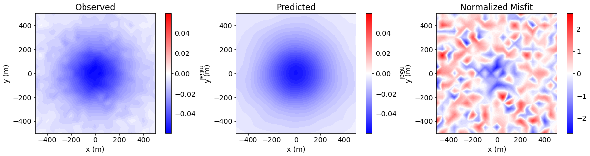
Data Misfit#
Show code cell source
data_array = np.c_[grav_data.dobs, dpred, (grav_data.dobs-dpred)/grav_data.standard_deviation]

fig = plt.figure(figsize=(17, 4))
plot_title = ["Observed", "Predicted", "Normalized Misfit"]
plot_units = ["mGal", "nGal", ""]

ax1 = 3 * [None]
ax2 = 3 * [None]
norm = 3 * [None]
cbar = 3 * [None]
cplot = 3 * [None]
v_lim = [
    np.max(np.abs(grav_data.dobs)),
    np.max(np.abs(grav_data.dobs)),
    np.max(np.abs(data_array[:, 2]))
]

for ii in range(0, 3):

    ax1[ii] = fig.add_axes([0.33 * ii + 0.03, 0.11, 0.25, 0.84])
    cplot[ii] = plot2Ddata(
        xyz,
        data_array[:, ii],
        ax=ax1[ii],
        ncontour=50,
        clim=(-v_lim[ii], v_lim[ii]),
        contourOpts={"cmap": "bwr"}
    )
    ax1[ii].set_title(plot_title[ii])
    ax1[ii].set_xlabel("x (m)")
    ax1[ii].set_ylabel("y (m)")

    ax2[ii] = fig.add_axes([0.33 * ii + 0.27, 0.11, 0.01, 0.84])
    norm[ii] = mpl.colors.Normalize(vmin=-v_lim[ii], vmax=v_lim[ii])
    cbar[ii] = mpl.colorbar.ColorbarBase(
        ax2[ii], norm=norm[ii], orientation="vertical", cmap=mpl.cm.bwr
    )
    cbar[ii].set_label(plot_units[ii], rotation=270, labelpad=15, size=12)

plt.show()
Comparing True and Recovered Models#
Show code cell source
fig = plt.figure(figsize=(9, 9))
font_size = 14

models_list = [true_model, simpeg_model]
titles_list = ['True Model', 'SimPEG Model']
ax1 = 2*[None]
cplot = 2*[None]
ax2 = 2*[None]
cbar = 2*[None]

for qq in range(0, 2):
    ax1[qq] = fig.add_axes([0.1, 0.55 - 0.5*qq, 0.78, 0.38])

    cplot[qq] = mesh.plot_slice(
        models_list[qq], normal='Y', ind=int(mesh.shape_cells[1]/2), grid=False, ax=ax1[qq]
    )
    cplot[qq][0].set_clim((np.min(models_list[qq]), np.max(models_list[qq])))
    ax1[qq].set_xlim([-800, 800])
    ax1[qq].set_ylim([-800, 0])
    ax1[qq].set_xlabel("X [m]", fontsize=font_size)
    ax1[qq].set_ylabel("Z [m]", fontsize=font_size, labelpad=-5)
    ax1[qq].tick_params(labelsize=font_size - 2)
    ax1[qq].set_title(titles_list[qq], fontsize=font_size + 2)

    ax2[qq] = fig.add_axes([0.9, 0.55 - 0.5*qq, 0.05, 0.38])
    norm = mpl.colors.Normalize(vmin=np.min(models_list[qq]), vmax=np.max(models_list[qq]))
    cbar[qq] = mpl.colorbar.ColorbarBase(
        ax2[qq], norm=norm, orientation="vertical"
    )
    cbar[qq].set_label(
        "$g/cm^3$",
        rotation=270,
        labelpad=20,
        size=font_size,
)

plt.show()