Gradiometry Simulation: Block in Halfspace

Geoscientific Problem

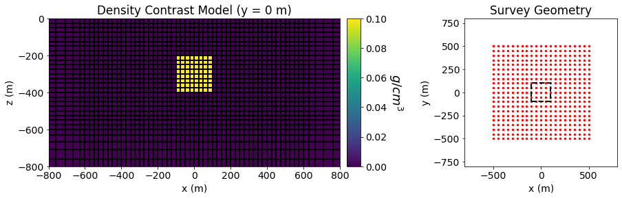
For this code comparison, we simulated gravity gradiometry data for a density contrast model over a dense block within a homogeneous background. The background density contrast was 0 \(g/cm^3\) and the density contrast of the block 0.1 \(g/cm^3\). The dimensions of the block in the x, y and z directions were are all 200 m. The block was buried at a depth of 200 m.

Gradiometry data were simulated 1 m above the surface. The survey region was 1000 m by 1000 m, the center of which lied directly over the center of the block. The station spacing was 50 m in both the X and Y directions.

A figure illustrating the density contrast model and survey geometry is shown further down

Codes/Formulations Being Compared

SimPEG 3D Integral Formulation: This approach to solving the forward problem uses the SimPEG.potential_fields.gravity.simulation.Simulation3DIntegral simulation class.

UBC-GIF GG3D v6.0.1: GG3D v6.0.1 is a voxel cell gravity gradiometry forward modeling and inversion package developed by the UBC Geophysical Inversion Facility. This software is proprietary and can ONLY be acquired through appropriate academic or commerical licenses. The numerical approach of the forward simulation is described in the online manual’s theory section. If you have a valid license, there are instructions for reproducing the results (add link).

Loading Assets Into the SimPEG Framework

We start by importing any necessary packages for running the notebook.

Show code cell source Hide code cell source

from SimPEG.utils import plot2Ddata
from SimPEG.utils.io_utils import read_gg3d_ubc
from discretize import TensorMesh
import matplotlib as mpl
import matplotlib.pyplot as plt
import numpy as np

mpl.rcParams.update({"font.size": 14})

Next we download the mesh, model and simulated data for each code.

Show code cell source Hide code cell source

# For each package, download .tar files

The mesh, model and predicted data for each code are then loaded into the SimPEG framework for plotting.

Show code cell source Hide code cell source

rootdir = './../../../assets/gravity/block_halfspace_gradiometry_fwd_simpeg/'
mesh_simpeg = TensorMesh.read_UBC(rootdir+'mesh.txt')
model_simpeg = TensorMesh.read_model_UBC(mesh_simpeg, rootdir+'model.den')
data_simpeg = read_gg3d_ubc(rootdir+'dpred_simpeg.gg')

rootdir = './../../../assets/gravity/block_halfspace_gradiometry_fwd_gg3d/'
mesh_ubc = TensorMesh.read_UBC(rootdir+'mesh.txt')
model_ubc = TensorMesh.read_model_UBC(mesh_simpeg, rootdir+'model.den')
data_ubc = read_gg3d_ubc(rootdir+'ggfor3d.gg')

Geophysical Scenario

Below, we plot the density contrast model and survey geometry used in the forward simulation.

Show code cell source Hide code cell source

fig = plt.figure(figsize=(14, 4))

ax11 = fig.add_axes([0.1, 0.15, 0.42, 0.75])
ind = int(mesh_simpeg.shape_cells[1]/2)
mesh_simpeg.plot_slice(
    model_simpeg, normal='Y', ind=ind, grid=True, ax=ax11, pcolor_opts={"cmap": "viridis"}
)

ax11.set_xlim([-800, 800])
ax11.set_ylim([-800, 0])
ax11.set_title("Density Contrast Model (y = 0 m)")
ax11.set_xlabel("x (m)")
ax11.set_ylabel("z (m)")

ax12 = fig.add_axes([0.53, 0.15, 0.02, 0.75])
norm = mpl.colors.Normalize(vmin=0, vmax=np.max(model_simpeg))
cbar = mpl.colorbar.ColorbarBase(
    ax12, norm=norm, cmap=mpl.cm.viridis, orientation="vertical"
)
cbar.set_label("$g/cm^3$", rotation=270, labelpad=25, size=18)

xyz = data_simpeg.survey.receiver_locations
ax21 = fig.add_axes([0.7, 0.15, 0.22, 0.75])
ax21.scatter(xyz[:, 0], xyz[:, 1], 6, 'r')
ax21.plot(100*np.r_[-1, 1, 1, -1, -1], 100*np.r_[-1, -1, 1, 1, -1], 'k--', lw=2.)
ax21.set_xlim([-800, 800])
ax21.set_ylim([-800, 800])
ax21.set_title("Survey Geometry")
ax21.set_xlabel("x (m)")
ax21.set_ylabel("y (m)")

Text(0, 0.5, 'y (m)')

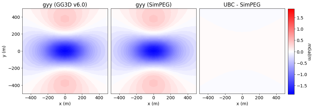
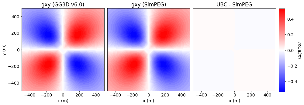
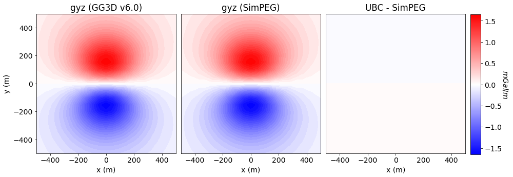
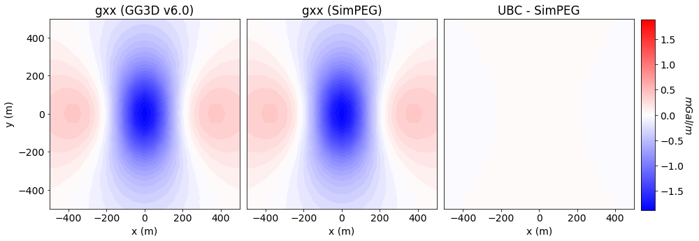
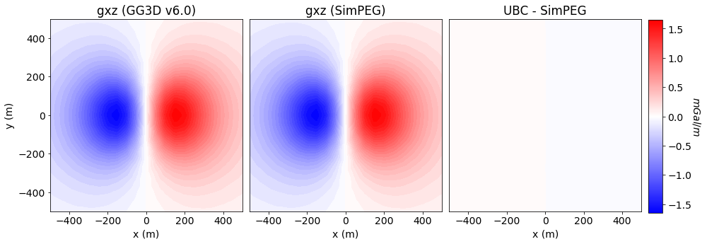
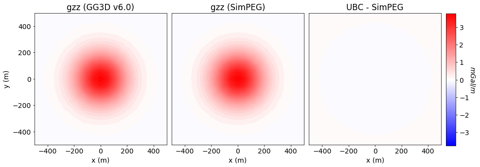
Simulated Data Plots

Here we plot the simulated data for all codes/formulations.

Show code cell source Hide code cell source

comp_str = list(data_simpeg.survey.components.keys())
xyz = data_simpeg.survey.receiver_locations
dpred_simpeg = np.reshape(data_simpeg.dobs, (data_simpeg.survey.nRx, len(comp_str)))
dpred_ubc = np.reshape(data_ubc.dobs, (data_ubc.survey.nRx, len(comp_str)))

for ii in range(0, len(comp_str)):
    
    max_val = np.max(np.abs(np.r_[
        dpred_ubc[:, ii], dpred_simpeg[:, ii], dpred_ubc[:, ii]-dpred_simpeg[:, ii]
    ]))

    fig = plt.figure(figsize=(14, 5))

    ax1 = fig.add_axes([0.05, 0.1, 0.27, 0.85])
    plot2Ddata(
        xyz, dpred_ubc[:, ii], ax=ax1, clim=(-max_val, max_val),
        ncontour=50, contourOpts={"cmap": "bwr"}
    )
    ax1.set_title(comp_str[ii] + " (GG3D v6.0)")
    ax1.set_xlabel("x (m)")
    ax1.set_ylabel("y (m)")

    ax2 = fig.add_axes([0.33, 0.1, 0.27, 0.85])
    plot2Ddata(
        xyz, dpred_simpeg[:, ii], ax=ax2, clim=(-max_val, max_val),
        ncontour=50, contourOpts={"cmap": "bwr"}
    )
    ax2.set_title(comp_str[ii] + " (SimPEG)")
    ax2.set_xlabel("x (m)")
    ax2.set_yticks([])

    ax3 = fig.add_axes([0.61, 0.1, 0.27, 0.85])
    plot2Ddata(
        xyz, dpred_ubc[:, ii]-dpred_simpeg[:, ii], ax=ax3,
        clim=(-max_val, max_val), ncontour=50, contourOpts={"cmap": "bwr"}
    )
    ax3.set_title("UBC - SimPEG")
    ax3.set_xlabel("x (m)")
    ax3.set_yticks([])

    ax4 = fig.add_axes([0.89, 0.14, 0.02, 0.76])
    norm = mpl.colors.Normalize(vmin=-max_val, vmax=max_val)
    cbar = mpl.colorbar.ColorbarBase(
        ax4, norm=norm, orientation="vertical", cmap=mpl.cm.bwr
    )
    cbar.set_label("$mGal/m$", rotation=270, labelpad=15, size=14)

    plt.show()