Reproduce: SimPEG#
Simulating Gradiometry Data Over a Block in a Halfspace#
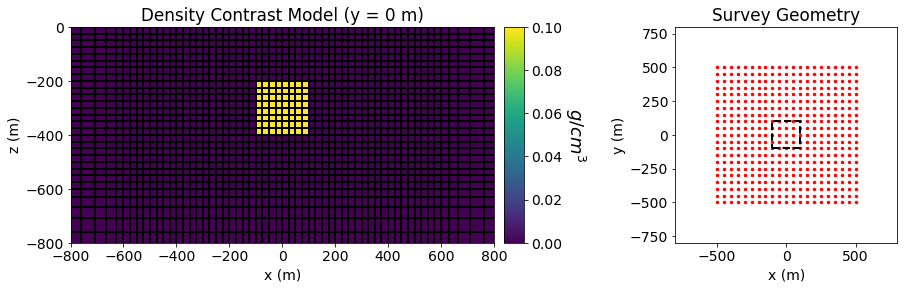
Gradiometry data are simulated for a density contrast model over block in a halfspace. The density contrast of the background is 0 \(g/cm^3\) and the density contrast of the block is 0.1 \(g/cm^3\). The dimensions of the block in the x, y and z directions are all 200 m. The block is buried at a depth of 200 m.
Gradiometry data are simulated on a regular grid of points at a heigh of 1 m above the Earth’s surface. The station spacing is 50 m in both the X and Y directions.
SimPEG Package Details#
Link to the docstrings for the simulation class. The docstrings will have a citation and show the integral equation.
Running the Forward Simulation#
We begin by loading all necessary packages and setting any global parameters for the notebook.
Show code cell source
from SimPEG import dask
from SimPEG.potential_fields import gravity
from SimPEG.utils import plot2Ddata
from SimPEG.utils.io_utils import read_gg3d_ubc, write_gg3d_ubc
from SimPEG import maps, data
from discretize import TensorMesh
import matplotlib as mpl
import matplotlib.pyplot as plt
import numpy as np

mpl.rcParams.update({"font.size": 14})
write_output = True
A compressed folder containing the assets required to run the notebook is then downloaded. This includes mesh, model and survey files for the forward simulation.
Show code cell source
# Download .tar files
Extracted files are then loaded into the SimPEG framework.
Show code cell source
rootdir = './../../../assets/gravity/block_halfspace_gradiometry_fwd_simpeg/'
meshfile = rootdir + 'mesh.txt'
modelfile = rootdir + 'model.den'
locfile = rootdir + 'survey.loc'

mesh = TensorMesh.read_UBC(meshfile)
model = TensorMesh.read_model_UBC(mesh, modelfile)
grav_data = read_gg3d_ubc(locfile)
Below, we plot the model and the survey geometry used in the forward simulation.
Show code cell source
fig = plt.figure(figsize=(14, 4))

ax11 = fig.add_axes([0.1, 0.15, 0.42, 0.75])
ind = int(mesh.shape_cells[1]/2)
mesh.plot_slice(
    model, normal='Y', ind=ind, grid=True, ax=ax11, pcolor_opts={"cmap": "viridis"}
)

ax11.set_xlim([-800, 800])
ax11.set_ylim([-800, 0])
ax11.set_title("Density Contrast Model (y = 0 m)")
ax11.set_xlabel("x (m)")
ax11.set_ylabel("z (m)")

ax12 = fig.add_axes([0.53, 0.15, 0.02, 0.75])
norm = mpl.colors.Normalize(vmin=0, vmax=np.max(model))
cbar = mpl.colorbar.ColorbarBase(
    ax12, norm=norm, cmap=mpl.cm.viridis, orientation="vertical"
)
cbar.set_label("$g/cm^3$", rotation=270, labelpad=25, size=18)

xyz = grav_data.survey.receiver_locations
ax21 = fig.add_axes([0.7, 0.15, 0.22, 0.75])
ax21.scatter(xyz[:, 0], xyz[:, 1], 6, 'r')
ax21.plot(100*np.r_[-1, 1, 1, -1, -1], 100*np.r_[-1, -1, 1, 1, -1], 'k--', lw=2.)
ax21.set_xlim([-800, 800])
ax21.set_ylim([-800, 800])
ax21.set_title("Survey Geometry")
ax21.set_xlabel("x (m)")
ax21.set_ylabel("y (m)")
Text(0, 0.5, 'y (m)')
Here we define the mapping from the model to the mesh, extract the survey from the data object and define the forward simulation.
rho_map = maps.IdentityMap(nP=mesh.nC)

survey = grav_data.survey

simulation = gravity.simulation.Simulation3DIntegral(
    survey=survey,
    mesh=mesh,
    rhoMap=rho_map,
    store_sensitivities="forward_only"
)
Finally, we predict the gradiometry data for the density contrast model provided.
dpred_simpeg = simulation.dpred(model)
Forward calculation:
[########################################] | 100% Completed |  3min 37.6s
If desired, we can export the simulated gradiometry data to a UBC formatted data file.
if write_output:
    data_simpeg = data.Data(survey=survey, dobs=dpred_simpeg)
    outname = rootdir + 'dpred_simpeg.gg'
    write_gg3d_ubc(outname, data_simpeg)
Observation file saved to: ./../../../assets/gravity/block_halfspace_gradiometry_fwd_simpeg/dpred_simpeg.gg
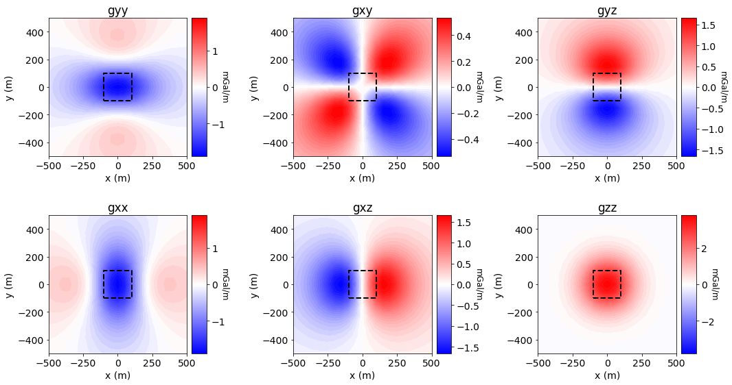
Plotting Simulated Gradiometry Data#
Show code cell source
component_name = list(data_simpeg.survey.components.keys())
xyz = survey.receiver_locations
data_plotting = np.reshape(dpred_simpeg, (survey.nRx, 6))

fig = plt.figure(figsize=(15, 8))

ax1 = 6 * [None]
ax2 = 6 * [None]
norm = 6 * [None]
cbar = 6 * [None]
cplot = 6 * [None]

COUNT = 0
for ii in range(0, 2):
    for jj in range(0, 3):
        v_lim = np.max(np.abs(data_plotting[:, COUNT]))

        ax1[COUNT] = fig.add_axes([0.05+0.33*jj, 0.6-0.5*ii, 0.22, 0.35])
        cplot[COUNT] = plot2Ddata(
            xyz, data_plotting[:, COUNT], ax=ax1[COUNT], clim=(-v_lim, v_lim),
            ncontour=50, contourOpts={"cmap": "bwr"}
        )
        ax1[COUNT].plot(100*np.r_[-1, 1, 1, -1, -1], 100*np.r_[-1, -1, 1, 1, -1], 'k--', lw=2.)
        ax1[COUNT].set_title(component_name[COUNT])
        ax1[COUNT].set_xlabel("x (m)")
        ax1[COUNT].set_ylabel("y (m)")

        ax2[COUNT] = fig.add_axes([0.26+0.33*jj, 0.6-0.5*ii, 0.02, 0.35])
        norm[COUNT] = mpl.colors.Normalize(vmin=-v_lim, vmax=v_lim)
        cbar[COUNT] = mpl.colorbar.ColorbarBase(
            ax2[COUNT], norm=norm[COUNT], orientation="vertical", cmap=mpl.cm.bwr
        )
        cbar[COUNT].set_label('mGal/m', rotation=270, labelpad=5, size=12)

        COUNT += 1

plt.show()