Reproduce: SimPEG OcTree#
Simulating Pole-Dipole IP Data over a Conductive and a Resistive Block#
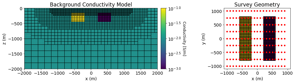
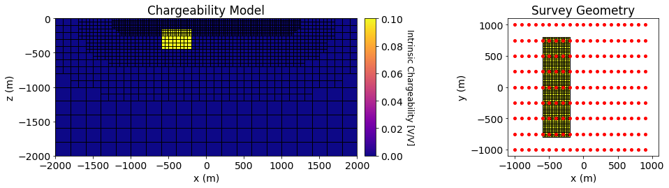
Pole-dipole induced polarization data are simulated over a conductive and chargeable block and over a resistive block. The background is non-chargeable and has a conductivity is \(\sigma_0\) = 0.01 S/m. The conductive-chargeable block has a conductivity of \(\sigma_c\) = 0.1 S/m and an intrinsic chargeability of \(\eta_c\) = 0.1 V/V. The resistor is non-chargeable and has a conductivity of \(\sigma_r\) = 0.001 S/m. Both blocks are oriented along the Northing direction and have x, y and z dimensions of 400 m, 1600 m and 320 m. Both blocks are buried at a depth of 160 m.
Apparent chargeability data are simulated with a pole-dipole configuration. The survey consists of 9 West-East survey lines, each with a length of 2000 m. The line spacing is 250 m and the electrode spacing is 100 m.
SimPEG Package Details¶#
Link to the docstrings for the simulation class.
Running the Forward Simulation#
We begin by loading all necessary packages and setting any global parameters for the notebook.
Show code cell source
from SimPEG import dask
from SimPEG.electromagnetics.static import induced_polarization as ip
from SimPEG.electromagnetics.static.utils.static_utils import plot_3d_pseudosection, apparent_resistivity
from SimPEG.utils.io_utils import read_dcipoctree_ubc, write_dcipoctree_ubc
from SimPEG import maps, data
from discretize import TreeMesh
import matplotlib as mpl
import matplotlib.pyplot as plt
import plotly
import numpy as np
from pymatsolver import Pardiso

mpl.rcParams.update({"font.size": 14})
write_output = True
A compressed folder containing the assets required to run the notebook is then downloaded. This includes mesh, model and survey files for the forward simulation.
Show code cell source
rootdir = './../../../assets/dcip/block_model_ip_fwd_simpeg_octree/'
meshfile = rootdir + 'octree_mesh.txt'
confile = rootdir + 'true_model.con'
chgfile = rootdir + 'true_model.chg'
locfile = rootdir + 'survey.loc'

mesh = TreeMesh.readUBC(meshfile)
conductivity_model = TreeMesh.readModelUBC(mesh, confile)
chargeability_model = TreeMesh.readModelUBC(mesh, chgfile)
ip_data = read_dcipoctree_ubc(locfile, 'apparent_chargeability')
Below, we plot the background conductivity model, the chargeability model and the survey geometry used in the forward simulation.
Show code cell source
vmin = np.log10(conductivity_model.min())
vmax = np.log10(conductivity_model.max())
ind = int(len(mesh.hy)/2)

fig = plt.figure(figsize=(15, 3.5))

ax1 = fig.add_axes([0.1, 0.12, 0.4, 0.78])
mesh.plotSlice(
    np.log10(conductivity_model), ax=ax1, normal='Y', grid=True,
    ind=ind, clim=(vmin, vmax), pcolorOpts={"cmap": "viridis"},
)
ax1.set_xlim([-2000, 2000])
ax1.set_ylim([-2000, 0])
ax1.set_title("Background Conductivity Model")
ax1.set_xlabel("x (m)")
ax1.set_ylabel("z (m)")

ax2 = fig.add_axes([0.51, 0.12, 0.015, 0.78])
norm = mpl.colors.Normalize(
    vmin=vmin, vmax=vmax
)
cbar = mpl.colorbar.ColorbarBase(
    ax2, norm=norm, cmap=mpl.cm.viridis, orientation="vertical", format="$10^{%.1f}$"
)
cbar.set_label("Conductivity [S/m]", rotation=270, labelpad=15, size=12)

ax3 = fig.add_axes([0.7, 0.12, 0.2, 0.78])
ind = int(len(mesh.hz)-10)
masked_model = np.log10(conductivity_model)
masked_model[masked_model==-2]=np.NaN
mesh.plot_slice(
    masked_model, ax=ax3, normal='Z', grid=True,
    ind=ind, clim=(vmin, vmax), pcolorOpts={"cmap": "viridis"},
)
for ii in range(0, 9):
    ax3.plot(np.arange(-1000, 1000, 100), -1000+ii*250*np.ones(20), 'ro', markersize=4)
ax3.set_xlim([-1100, 1100])
ax3.set_ylim([-1100, 1100])
ax3.set_xlabel('x (m)')
ax3.set_ylabel('y (m)')
ax3.set_title('Survey Geometry')

plt.show()


vmin = chargeability_model.min()
vmax = chargeability_model.max()
ind = int(len(mesh.hy)/2)

fig = plt.figure(figsize=(15, 3.5))
ax1 = fig.add_axes([0.1, 0.12, 0.4, 0.78])
mesh.plotSlice(
    chargeability_model, ax=ax1, normal='Y',grid=True, ind=ind,
    clim=(vmin, vmax), pcolorOpts={"cmap": "plasma"},
)
ax1.set_xlim([-2000, 2000])
ax1.set_ylim([-2000, 0])
ax1.set_title("Chargeability Model")
ax1.set_xlabel("x (m)")
ax1.set_ylabel("z (m)")

ax2 = fig.add_axes([0.51, 0.12, 0.015, 0.78])
norm = mpl.colors.Normalize(
    vmin=vmin, vmax=vmax
)
cbar = mpl.colorbar.ColorbarBase(
    ax2, norm=norm, cmap=mpl.cm.plasma, orientation="vertical", format="${%.2f}$"
)
cbar.set_label("Intrinsic Chargeability [V/V]", rotation=270, labelpad=15, size=12)

ax3 = fig.add_axes([0.7, 0.12, 0.2, 0.78])
ind = int(len(mesh.hz)-10)
masked_model = chargeability_model.copy()
masked_model[masked_model<0.1]=np.NaN
mesh.plot_slice(
    masked_model, ax=ax3, normal='Z', grid=True,
    ind=ind, clim=(vmin, vmax), pcolorOpts={"cmap": "plasma"},
)
for ii in range(0, 9):
    ax3.plot(np.arange(-1000, 1000, 100), -1000+ii*250*np.ones(20), 'ro', markersize=4)
ax3.set_xlim([-1100, 1100])
ax3.set_ylim([-1100, 1100])
ax3.set_xlabel('x (m)')
ax3.set_ylabel('y (m)')
ax3.set_title('Survey Geometry')

plt.show()
Here we define the mapping from the model to the mesh, extract the survey from the data object and define the forward simulation.
Show code cell source
chargeability_map = maps.IdentityMap()

ip_survey = ip_data.survey

ip_simulation = ip.simulation.Simulation3DNodal(
    mesh, survey=ip_survey, etaMap=chargeability_map, solver=Pardiso,
    sigma=conductivity_model, verbose=True, bc_type='Neumann'
)
Homogeneous Neumann is the natural BC for this nodal discretization.
Finally, we predict apparent chargeability data for the chargeability model provided.
Show code cell source
dpred_simpeg = ip_simulation.dpred(chargeability_model)
>> Solve DC problem
>> Compute predicted data
If desired, we can export the simulated gravity data to a UBC formatted data file.
Show code cell source
if write_output:
    data_simpeg = data.Data(survey=ip_survey, dobs=dpred_simpeg)
    outname = rootdir + 'dpred_simpeg.txt'
    write_dcipoctree_ubc(outname, data_simpeg, 'apparent_chargeability', 'dpred')

    np.random.seed(83)
    standard_deviation = 0.001
    dobs = dpred_simpeg + standard_deviation * np.random.rand(len(dpred_simpeg))
    dobs_simpeg = data.Data(survey=ip_survey, dobs=dobs, standard_deviation=standard_deviation)
    outname = rootdir + 'dobs_simpeg.txt'
    write_dcipoctree_ubc(outname, dobs_simpeg, 'apparent_chargeability', 'dobs')
Apparent Chargeability Data Plot#
Show code cell source
mpl.rcParams.update({'font.size': 16})

plane_points = []
for x in np.arange(-1000, 1100, 500):
    p1, p2, p3 = np.array([-1000.,x,0]), np.array([1000,x,0]), np.array([1000,x,-1000])
    plane_points.append([p1,p2,p3])

scene_camera=dict(
    center=dict(x=-0.05, y=0, z=-0.2), eye=dict(x=1.1, y=-0.9, z=1.35)
)
scene = dict(
    xaxis=dict(range=[-1000, 1000]), yaxis=dict(range=[-1000, 1000]),
    zaxis=dict(range=[-500, 0]), aspectratio=dict(x=1, y=1, z=0.5)
)

vlim = [dpred_simpeg.min(), dpred_simpeg.max()]

fig1 = plot_3d_pseudosection(
    ip_survey, dpred_simpeg, scale='lin', vlim=vlim,
    plane_points=plane_points, plane_distance=10., units='V/V',
    marker_opts={"colorscale": "plasma"}
)

fig1.update_layout(
    title_text="Apparent Chargeability Data", title_x=0.5, width=800, height=700,
    scene_camera=scene_camera, scene=scene
)

plotly.io.show(fig1)