Reproduce: Analytic#
Simulating Transient Response over a Conductive Sphere#
Here we simulate the transient response from a conductive sphere in a vacuum. The sphere has a conductivity of \(\sigma\) = 100 S/m. The center of the sphere is located at (0,0,-50) and has a radius of \(a\) = 8 m.
The transient response is simulated for x, y and z oriented magnetic dipoles at (-5, 0, 10). The x, y and z components of H and dB/dt are simulated at (5, 0, 10). However, we only plot the data for horizontal coaxial, horizontal coplanar and vertical coplanar geometries.
Package Details#
Wait and Spies analytic solution. See https://em.geosci.xyz/content/maxwell3_fdem/inductive_sources/sphere/index.html for a summary of the solution.
Reference: J. R. Wait. A conductive sphere in a time varying magnetic field. Geophysics, 16:666–672, 1951.
Reproducing the Forward Simulation Result#
We begin by loading all necessary packages and setting any global parameters for the notebook.
Show code cell source
from SimPEG.utils import mkvc
import numpy as np
import matplotlib as mpl
import matplotlib.pyplot as plt
from scipy.constants import mu_0
import scipy.special as spec

mpl.rcParams.update({"font.size": 14})
write_output = True
Define layered Earth model.
Show code cell source
rootdir = './../../../assets/tdem/sphere_vacuum_conductive_fwd_simpeg/'

a = 8                                # radius of sphere
sig0 = 1e-8                          # background conductivity
sig = 1e2                            # electrical conductivity of sphere
mur = 1                              # relative permeability of sphere
xyzs = np.c_[0., 0., -50.]           # xyz location of the sphere
Here, we define the survey geometry for the forward simulation.
Show code cell source
xyz_tx = np.c_[-5., 0., 10.]         # Transmitter location
xyz_rx = np.c_[5., 0., 10.]          # Receiver location
times = np.logspace(-5,-2,10)        # Times
tx_moment = 1                        # Dipole moment
Here we define some functions required for the forward simulation.
Show code cell source
def compute_primary_field_dipole(orientation, pxyz, qxyz):
    """
    For an X, Y or Z orientationed magnetic dipole, compute the free-space primary field for a dipole moment of 1.

    orientation: 'x', 'y' or 'z'
    pxyz : [x,y,z] locations of the dipole transmitters
    qxyz : [x,y,z] location at the centre location of the sphere

    """

    R = np.sqrt((qxyz[0] - pxyz[:,0]) ** 2 + (qxyz[1] - pxyz[:,1]) ** 2 + (qxyz[2] - pxyz[:,2]) ** 2)

    if orientation == "x":
        Hpx = (1 / (4 * np.pi)) * (3 * (qxyz[0] - pxyz[:,0]) * (qxyz[0] - pxyz[:,0]) / R ** 5 - 1 / R ** 3)
        Hpy = (1 / (4 * np.pi)) * (3 * (qxyz[1] - pxyz[:,1]) * (qxyz[0] - pxyz[:,0]) / R ** 5)
        Hpz = (1 / (4 * np.pi)) * (3 * (qxyz[2] - pxyz[:,2]) * (qxyz[0] - pxyz[:,0]) / R ** 5)
    elif orientation == "y":
        Hpx = (1 / (4 * np.pi)) * (3 * (qxyz[0] - pxyz[:,0]) * (qxyz[1] - pxyz[:,1]) / R ** 5)
        Hpy = (1 / (4 * np.pi)) * (3 * (qxyz[1] - pxyz[:,1]) * (qxyz[1] - pxyz[:,1]) / R ** 5 - 1 / R ** 3)
        Hpz = (1 / (4 * np.pi)) * (3 * (qxyz[2] - pxyz[:,2]) * (qxyz[1] - pxyz[:,1]) / R ** 5)
    elif orientation == "z":
        Hpx = (1 / (4 * np.pi)) * (3 * (qxyz[0] - pxyz[:,0]) * (qxyz[2] - pxyz[:,2]) / R ** 5)
        Hpy = (1 / (4 * np.pi)) * (3 * (qxyz[1] - pxyz[:,1]) * (qxyz[2] - pxyz[:,2]) / R ** 5)
        Hpz = (1 / (4 * np.pi)) * (3 * (qxyz[2] - pxyz[:,2]) * (qxyz[2] - pxyz[:,2]) / R ** 5 - 1 / R ** 3)

    return np.c_[Hpx, Hpy, Hpz]


def compute_dipolar_response(m, pxyz, qxyz):
    """
    For a sphere with dipole moment [mx, my, mz], compute the dipolar response

    m : dipole moments [mx, my, mz]
    orientation of the receiver: 'x', 'y' or 'z'
    pxyz : [x,y,z] locations of the receivers
    qxyz : [x,y,z] location at the centre location of the sphere

    """

    R = np.sqrt((qxyz[:,0] - pxyz[:,0]) ** 2 + (qxyz[:,1] - pxyz[:,1]) ** 2 + (qxyz[:,2] - pxyz[:,2]) ** 2)

    Hx = (1 / (4 * np.pi)) * ( 3 * (pxyz[:,0] - qxyz[:,0]) * (
                m[:,0]*(pxyz[:,0] - qxyz[:,0]) +
                m[:,1]*(pxyz[:,1] - qxyz[:,1]) +
                m[:,2]*(pxyz[:,2] - qxyz[:,2])
            ) / R ** 5 - m[:,0] / R ** 3)

    Hy = (1 / (4 * np.pi)) * ( 3 * (pxyz[:,1] - qxyz[:,1]) * (
                m[:,0]*(pxyz[:,0] - qxyz[:,0]) +
                m[:,1]*(pxyz[:,1] - qxyz[:,1]) +
                m[:,2]*(pxyz[:,2] - qxyz[:,2])
            ) / R ** 5 - m[:,1] / R ** 3)

    Hz = (1 / (4 * np.pi)) * ( 3 * (pxyz[:,2] - qxyz[:,2]) * (
                m[:,0]*(pxyz[:,0] - qxyz[:,0]) +
                m[:,1]*(pxyz[:,1] - qxyz[:,1]) +
                m[:,2]*(pxyz[:,2] - qxyz[:,2])
            ) / R ** 5 - m[:,2] / R ** 3)

    return np.c_[Hx, Hy, Hz]

def compute_coefficients(N):

    eta = np.pi*np.linspace(1,N,N)
    for ii in range(0, 20):
        eta = np.pi*np.linspace(1,N,N) + np.arctan(((mur - 1)*eta)/(mur - 1 + eta**2))

    return eta


def compute_excitation_factor(t, eta, sig, mur, a):
    """
    Compute Excitation Factor (FEM)

    t : times
    eta : coefficients
    sig : conductivity
    mur : relative permeability
    a : radius
    """

    alpha = (mur + 2)*(mur - 1)
    beta = np.sqrt(4*np.pi*1e-7*mur*sig)*a

    chi = len(t)*[None]
    for ii in range(0, len(t)):
        chi[ii] = 9 * mur * np.sum(
            np.exp(-t[ii] * eta**2 / beta**2) / (alpha + eta**2)
        )

    return chi


def compute_excitation_factor_derivative(t, eta, sig, mur, a):
    """
    Compute Excitation Factor (FEM)

    t : times
    eta : coefficients
    sig : conductivity
    mur : relative permeability
    a : radius
    """

    alpha = (mur + 2)*(mur - 1)
    beta = np.sqrt(4*np.pi*1e-7*mur*sig)*a

    dchi = len(t)*[None]
    for ii in range(0, len(t)):
        dchi[ii] = -(9 * mur / beta**2) * np.sum(
            eta**2 * np.exp(-t[ii] * eta**2 / beta**2) / (alpha + eta**2)
        )

    return dchi
Finally, we simulate the predicted data.
Show code cell source
# Compute coefficients
eta = compute_coefficients(500)

H_analytic = []
dBdt_analytic = []

for ii, comp in enumerate(['x','y','z']):

    # Compute the free space primary field at the location of the sphere
    Hp = mkvc(tx_moment*compute_primary_field_dipole(comp, xyz_tx, mkvc(xyzs)))

    # Compute dipole moment and its time derivative
    chi = compute_excitation_factor(times, eta, sig, mur, a)
    dchi = compute_excitation_factor_derivative(times, eta, sig, mur, a)
    m = (4*np.pi*a**3/3) * np.outer(chi, Hp)
    dmdt = (4*np.pi*a**3/3) * np.outer(dchi, Hp)

    # Predict data
    H_analytic.append(compute_dipolar_response(m, xyz_rx, xyzs))
    dBdt_analytic.append(mu_0*compute_dipolar_response(dmdt, xyz_rx, xyzs))
We can export the data.
Show code cell source
if write_output:

    fname_analytic = rootdir + 'dpred_analytic.txt'

    header = 'TIME HX HY HZ DBDTX DBDTY DBDTZ'

    t_column = np.kron(np.ones(3), times)

    dpred_analytic = np.c_[t_column, np.vstack(H_analytic), np.vstack(dBdt_analytic)]

    fid = open(fname_analytic, 'w')
    np.savetxt(fid, dpred_analytic, fmt='%.6e', delimiter=' ', header=header)
    fid.close()
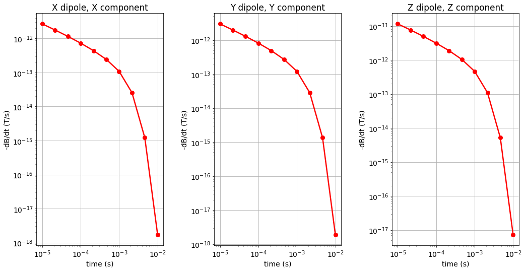
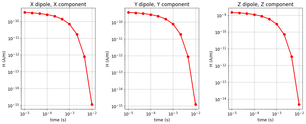
Plotting Simulated Data#
Here, we plot the H and dB/dt data for horizontal coaxial, horizontal coplanar and vertical coplanar geometries.
Show code cell source
fig = plt.figure(figsize=(14, 6))
lw = 2.5
ms = 8

ax1 = 3*[None]

for ii, comp in enumerate(['X','Y','Z']):

    ax1[ii] = fig.add_axes([0.05+0.35*ii, 0.1, 0.25, 0.8])
    ax1[ii].loglog(times, H_analytic[ii][:, ii], 'r-o', lw=lw, markersize=8)
    ax1[ii].set_xticks([1e-5, 1e-4, 1e-3, 1e-2])
    ax1[ii].grid()
    ax1[ii].set_xlabel('time (s)')
    ax1[ii].set_ylabel('H (A/m)'.format(comp))
    ax1[ii].set_title(comp + ' dipole, ' + comp + ' component')
Show code cell source
fig = plt.figure(figsize=(14, 8))
lw = 2.5
ms = 8

ax1 = 3*[None]

for ii, comp in enumerate(['X','Y','Z']):

    ax1[ii] = fig.add_axes([0.05+0.35*ii, 0.1, 0.25, 0.8])
    ax1[ii].loglog(times, -dBdt_analytic[ii][:, ii], 'r-o', lw=lw, markersize=8)
    ax1[ii].set_xticks([1e-5, 1e-4, 1e-3, 1e-2])
    ax1[ii].grid()
    ax1[ii].set_xlabel('time (s)')
    ax1[ii].set_ylabel('-dB/dt (T/s)'.format(comp))
    ax1[ii].set_title(comp + ' dipole, ' + comp + ' component')