TMI Inversion: Block in Halfspace (Smooth)#
Geoscientific Problem#
For this code comparison, we inverted total magnetic intensity (TMI) data collected over a block within a homogeneous halfspace. For each coding package, we invert for the smoothest model using an unconstrained least-squares inversion approach.
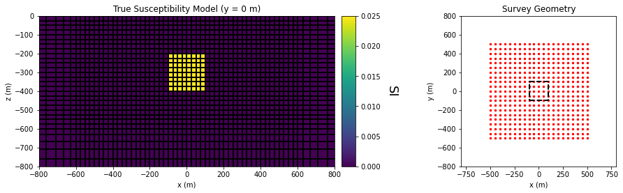
The true model consists of a susceptible block (0.025 SI) within a minimally susceptible halfspace (0.0001 SI). The dimensions of the block in the x, y and z directions were are all 200 m. The block was buried at a depth of 200 m. The Earth’s inducing field had an inclination of 65 degrees, a declination of 25 degrees and an intensity of 50,000 nT.
The data being inverted were generated using the UBC MAG3D v6.0.1 code. Synthetic TMI data were simulated within a 1000 m by 1000 m region at an elevation of 30 m; the center of which lied directly over the center of the block. The station spacing was 50 m in both the X and Y directions. Observed data were sythnetically created by adding Gaussian noise with a standard deviation of 1 nT to the simulated data. A floor uncertainty of 1 nT was assigned to the observed data.
Codes/Formulations Being Compared#
SimPEG 3D Integral Formulation: This approach to solving the forward problem uses the SimPEG.potential_fields.magnetics.simulation.Simulation3DIntegral simulation class.
UBC MAG3D v6.0: MAG3D v6.0 is a voxel cell magnetic forward modeling and inversion package developed by the UBC Geophysical Inversion Facility. This software is proprietary and can ONLY be acquired through appropriate academic or commerical licenses. The numerical approach of the forward simulation is described in the online manual’s theory section. If you have a valid license, there are instructions for reproducing the results (add link).
Loading Assets Into the SimPEG Framework#
We start by importing any necessary packages for running the notebook.
Show code cell source
from SimPEG.potential_fields import magnetics
from SimPEG.utils import plot2Ddata
from SimPEG.utils.io_utils import read_mag3d_ubc
from SimPEG import maps, data_misfit, regularization, optimization, inverse_problem, inversion, directives
from discretize import TensorMesh
import matplotlib as mpl
import matplotlib.pyplot as plt
import numpy as np
Next we download the mesh, true model, recovered model, predicted data and observed data for each coding package/formulation.
Show code cell source
# For each package, download .tar files
For each coding package/formulation, the assets are loaded into the SimPEG framework
Show code cell source
rootdir = './../../../assets/magnetics/block_halfspace_tmi_inv_smooth_simpeg/'
mesh_simpeg = TensorMesh.read_UBC(rootdir+'mesh.txt')
true_model_simpeg = TensorMesh.read_model_UBC(mesh_simpeg, rootdir+'true_model.sus')
recovered_model_simpeg = TensorMesh.read_model_UBC(mesh_simpeg, rootdir+'recovered_model.sus')
dobs_simpeg = read_mag3d_ubc(rootdir+'dobs.mag')
dpred_simpeg = read_mag3d_ubc(rootdir+'dpred.mag')

rootdir = './../../../assets/magnetics/block_halfspace_tmi_inv_smooth_mag3d/'
mesh_ubc = TensorMesh.read_UBC(rootdir+'mesh.txt')
true_model_ubc = TensorMesh.read_model_UBC(mesh_simpeg, rootdir+'true_model.sus')
recovered_model_ubc = TensorMesh.read_model_UBC(mesh_simpeg, rootdir+'maginv3d_002.sus')
dobs_ubc = read_mag3d_ubc(rootdir+'dobs.mag')
dpred_ubc = read_mag3d_ubc(rootdir+'maginv3d_002.pre')
True Model and Survey Geometry#
Show code cell source
fig = plt.figure(figsize=(14, 4))

ax11 = fig.add_axes([0.1, 0.15, 0.42, 0.75])
ind = int(mesh_simpeg.shape_cells[1]/2)
mesh_simpeg.plot_slice(
    true_model_simpeg, normal='Y', ind=ind, grid=True, ax=ax11, pcolor_opts={"cmap": "viridis"}
)

ax11.set_xlim([-800, 800])
ax11.set_ylim([-800, 0])
ax11.set_title("True Susceptibility Model (y = 0 m)")
ax11.set_xlabel("x (m)")
ax11.set_ylabel("z (m)")

ax12 = fig.add_axes([0.53, 0.15, 0.02, 0.75])
norm = mpl.colors.Normalize(vmin=0, vmax=np.max(true_model_simpeg))
cbar = mpl.colorbar.ColorbarBase(
    ax12, norm=norm, cmap=mpl.cm.viridis, orientation="vertical"
)
cbar.set_label("SI", rotation=270, labelpad=25, size=18)

xyz = dobs_simpeg.survey.receiver_locations
ax21 = fig.add_axes([0.7, 0.15, 0.22, 0.75])
ax21.scatter(xyz[:, 0], xyz[:, 1], 6, 'r')
ax21.plot(100*np.r_[-1, 1, 1, -1, -1], 100*np.r_[-1, -1, 1, 1, -1], 'k--', lw=2.)
ax21.set_xlim([-800, 800])
ax21.set_ylim([-800, 800])
ax21.set_title("Survey Geometry")
ax21.set_xlabel("x (m)")
ax21.set_ylabel("y (m)")
Text(0, 0.5, 'y (m)')
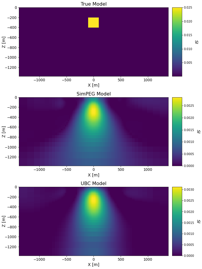
Comparing Recovered Models#
Show code cell source
fig = plt.figure(figsize=(9, 14))
font_size = 14

models_list = [true_model_simpeg, recovered_model_simpeg, recovered_model_ubc]
titles_list = ['True Model', 'SimPEG Model', 'UBC Model']
ax1 = 3*[None]
cplot = 3*[None]
ax2 = 3*[None]
cbar = 3*[None]

for qq in range(0, 3):
    ax1[qq] = fig.add_axes([0.1, 0.65 - 0.3*qq, 0.78, 0.23])

    cplot[qq] = mesh_simpeg.plot_slice(
        models_list[qq], normal='Y', ind=int(mesh_simpeg.shape_cells[1]/2), grid=False, ax=ax1[qq]
    )
    cplot[qq][0].set_clim((np.min(models_list[qq]), np.max(models_list[qq])))
    ax1[qq].set_xlabel("X [m]", fontsize=font_size)
    ax1[qq].set_ylabel("Z [m]", fontsize=font_size, labelpad=-5)
    ax1[qq].tick_params(labelsize=font_size - 2)
    ax1[qq].set_title(titles_list[qq], fontsize=font_size + 2)

    ax2[qq] = fig.add_axes([0.9, 0.65 - 0.3*qq, 0.05, 0.23])
    norm = mpl.colors.Normalize(vmin=np.min(models_list[qq]), vmax=np.max(models_list[qq]))
    cbar[qq] = mpl.colorbar.ColorbarBase(
        ax2[qq], norm=norm, orientation="vertical"
    )
    cbar[qq].set_label(
        "$SI$",
        rotation=270,
        labelpad=20,
        size=font_size,
)

plt.show()
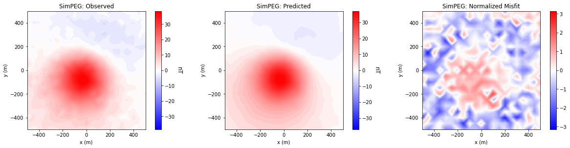
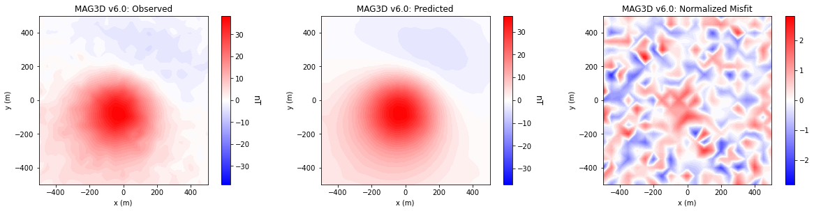
Comparing Data Misfits#
Show code cell source
data_array = [
    [
        dobs_simpeg.dobs,
        dpred_simpeg.dobs,
        (dobs_simpeg.dobs - dpred_simpeg.dobs) / dobs_simpeg.standard_deviation
    ], [
        dobs_ubc.dobs,
        dpred_ubc.dobs,
        (dobs_ubc.dobs - dpred_ubc.dobs) / dobs_ubc.standard_deviation
    ]
]
code_name = ['SimPEG', 'MAG3D v6.0']

for ii in range(0, len(data_array)):

    fig = plt.figure(figsize=(17, 4))

    plot_title = ["Observed", "Predicted", "Normalized Misfit"]
    plot_units = ["nT", "nT", ""]

    ax1 = 3 * [None]
    ax2 = 3 * [None]
    norm = 3 * [None]
    cbar = 3 * [None]
    cplot = 3 * [None]

    v_lim = [
        np.max(np.abs(data_array[ii][0])),
        np.max(np.abs(data_array[ii][1])),
        np.max(np.abs(data_array[ii][2]))
    ]

    for jj in range(0, 3):

        ax1[jj] = fig.add_axes([0.33 * jj + 0.03, 0.11, 0.25, 0.84])
        cplot[jj] = plot2Ddata(
            xyz,
            data_array[ii][jj],
            ax=ax1[jj],
            ncontour=50,
            clim=(-v_lim[jj], v_lim[jj]),
            contourOpts={"cmap": "bwr"}
        )
        ax1[jj].set_title(code_name[ii] + ': ' + plot_title[jj])
        ax1[jj].set_xlabel("x (m)")
        ax1[jj].set_ylabel("y (m)")

        ax2[jj] = fig.add_axes([0.33 * jj + 0.27, 0.11, 0.01, 0.84])
        norm[jj] = mpl.colors.Normalize(vmin=-v_lim[jj], vmax=v_lim[jj])
        cbar[jj] = mpl.colorbar.ColorbarBase(
            ax2[jj], norm=norm[jj], orientation="vertical", cmap=mpl.cm.bwr
        )
        cbar[jj].set_label(plot_units[jj], rotation=270, labelpad=15, size=12)

    plt.show()