Inductive Source Simulation: Conductive Sphere in Vacuum#
Geoscientific Problem#
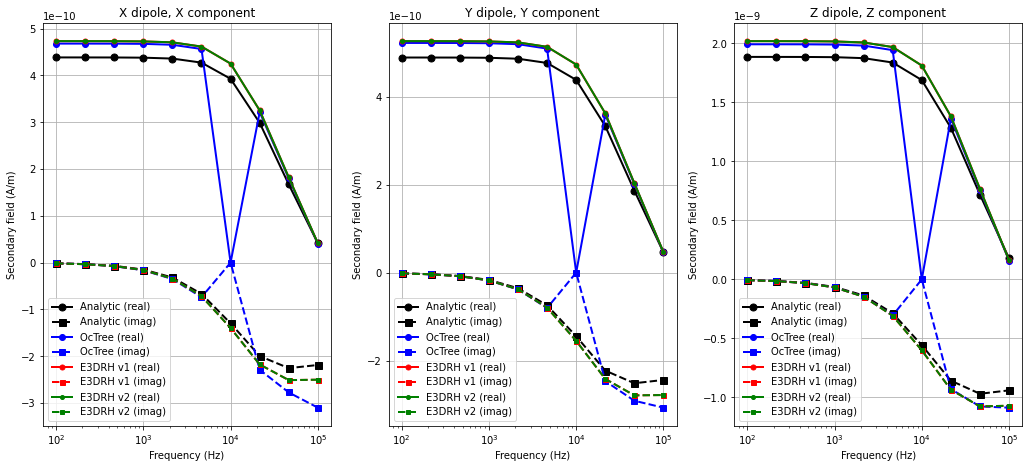
For this code comparison, we simulated secondary magnetic fields over a conductive and susceptible sphere in vacuum. The sphere had a conductivity of \(\sigma\) = 0.25 S/m and a susceptibility of \(\chi\) = 4 SI. The center of the sphere was located at (0,0,-50) and had a radius of \(a\) = 8 m.
Secondary magnetic fields were simulated for x, y and z oriented magnetic dipoles sources at (-5,0,10). The x, y and z components of the response were simulated for each source at (5,0,10). We plot only the horizontal coaxial, horizontal coplanar and vertical coplanar data.
Codes/Formulations Being Compared#
Analytic Solution: Wait and Spies analytic solution. See https://em.geosci.xyz/content/maxwell3_fdem/inductive_sources/sphere/index.html for a summary of the solution. Reference: J. R. Wait. A conductive sphere in a time varying magnetic field. Geophysics, 16:666–672, 1951.
SimPEG 3D OcTree Formulation (H-formulation):
UBC E3DRH v1: E3DRH v1 is a voxel cell FDEM forward modeling and inversion package developed by the UBC Geophysical Inversion Facility. This software is proprietary and can ONLY be acquired through appropriate commerical license. The numerical approach of the forward simulation is described in the online manual’s theory section. If you have a valid license, there are instructions for reproducing the results (add link).
UBC E3DRH v2: E3DRH v2 is a voxel cell FDEM forward modeling and inversion package developed by the UBC Geophysical Inversion Facility. This software is proprietary and can ONLY be acquired through appropriate commerical license. The numerical approach of the forward simulation is described in the online manual’s theory section. If you have a valid license, there are instructions for reproducing the results (add link).
Loading Assets Into the SimPEG Framework#
We start by importing any necessary packages for running the notebook.
Show code cell source
import numpy as np
import matplotlib as mpl
import matplotlib.pyplot as plt
from discretize import TreeMesh
from SimPEG import maps

mpl.rcParams.update({"font.size": 10})

frequencies = np.logspace(2, 5, 10)

plot_analytic = True
plot_simpeg_octree = True
plot_ubc_e3drh_v1 = True
plot_ubc_e3drh_v2 = True
Next we download the mesh, model and simulated data for each code.
Show code cell source
# For each package, download .tar files
The mesh, model and predicted data for each code are then loaded into the SimPEG framework for plotting.
Show code cell source
rootdir = './../../../assets/fdem/sphere_vacuum_susceptible_fwd'
mesh_simpeg = TreeMesh.read_UBC(rootdir+'_simpeg/octree_mesh.txt')
con_model_simpeg = TreeMesh.read_model_UBC(mesh_simpeg, rootdir+'_simpeg/model.con')
sus_model_simpeg = TreeMesh.read_model_UBC(mesh_simpeg, rootdir+'_simpeg/model.sus')

data_list = []
legend_str = []
style_list_real = ['k-o', 'b-o', 'r-o', 'g-o', 'c-o']
style_list_imag = ['k--s', 'b--s', 'r--s', 'g--s', 'c--s']

if plot_analytic:
    fname = '_simpeg/analytic.txt'
    data_array = np.loadtxt(rootdir+fname, skiprows=1)[:, 1:]
    data_array = np.reshape(data_array, (3, len(frequencies), 6))
    data_list.append(data_array)
    legend_str += ['Analytic (real)', 'Analytic (imag)']

if plot_simpeg_octree:
    fname = '_simpeg/dpred_octree.txt'
    data_array = np.loadtxt(rootdir+fname, skiprows=1)[:, 1:]
    data_array = np.reshape(data_array, (3, len(frequencies), 6))
    data_list.append(data_array)
    legend_str += ['OcTree (real)', 'OcTree (imag)']

if plot_ubc_e3drh_v1:
    fname = '_ubc_octree/fwd_v1/dpred_fwd.txt'
    d_e3dv1 = np.loadtxt(rootdir+fname, comments='%')
    d_e3dv1 = d_e3dv1[:, 9:15]  # extract Hx, Hy and Hz columns

    # Convert -iwt to +iwt
    d_e3dv1 = np.c_[
        d_e3dv1[:, 0], -d_e3dv1[:, 1],
        d_e3dv1[:, 2], -d_e3dv1[:, 3],
        d_e3dv1[:, 4], -d_e3dv1[:, 5]
    ]

    d_e3dv1 = np.reshape(d_e3dv1, (3, len(frequencies), 6))
    data_list.append(d_e3dv1)
    legend_str += ['E3DRH v1 (real)', 'E3DRH v1 (imag)']

if plot_ubc_e3drh_v2:
    fname = '_ubc_octree/fwd_v2/dpredFWD.txt'
    d_e3dv2 = np.loadtxt(rootdir+fname)

    # Extract Hx, Hy and Hz, and convert -iwt to +iwt
    d_e3dv2 = np.c_[
        d_e3dv2[0::3, 0], -d_e3dv2[0::3, 1],
        d_e3dv2[1::3, 0], -d_e3dv2[1::3, 1],
        d_e3dv2[2::3, 0], -d_e3dv2[2::3, 1]
    ]

    d_e3dv2 = np.reshape(d_e3dv2, (3, len(frequencies), 6))
    data_list.append(d_e3dv2)
    legend_str += ['E3DRH v2 (real)', 'E3DRH v2 (imag)']
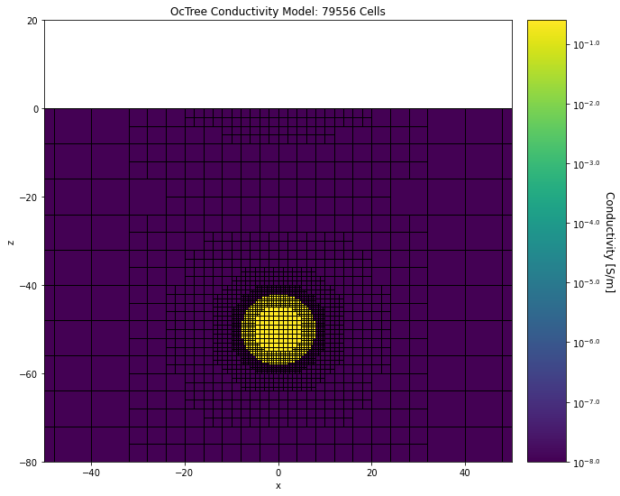
Plot Geophysical Scenario#
Below, we plot the conductivity model and survey geometry for the forward simulation.
Show code cell source
fig = plt.figure(figsize=(12,8))
ind_active = mesh_simpeg.cell_centers[:, 2] < 0
plotting_map = maps.InjectActiveCells(mesh_simpeg, ind_active, np.nan)
log_model = np.log10(con_model_simpeg[ind_active])

ax1 = fig.add_axes([0.14, 0.1, 0.6, 0.85])
mesh_simpeg.plot_slice(
    plotting_map * log_model,
    normal="Y", ax=ax1, ind=int(mesh_simpeg.h[1].size / 2), clim=(np.min(log_model), np.max(log_model)),
    grid=True
)

ax1.set_xlim([-50, 50])
ax1.set_ylim([-80, 20])
ax1.set_title("OcTree Conductivity Model: {} Cells".format(mesh_simpeg.nC))

ax2 = fig.add_axes([0.76, 0.1, 0.05, 0.85])
norm = mpl.colors.Normalize(
    vmin=np.min(log_model), vmax=np.max(log_model)
)
cbar = mpl.colorbar.ColorbarBase(
    ax2, norm=norm, orientation="vertical", format="$10^{%.1f}$"
)
cbar.set_label("Conductivity [S/m]", rotation=270, labelpad=15, size=12)
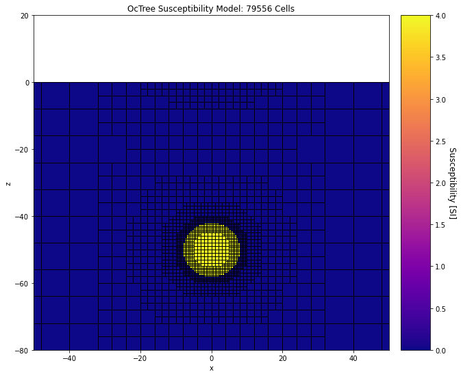
And here we plot the susceptibility model.
Show code cell source
fig = plt.figure(figsize=(12,8))

ax1 = fig.add_axes([0.14, 0.1, 0.6, 0.85])
mesh_simpeg.plot_slice(
    plotting_map * sus_model_simpeg[ind_active], normal="Y", ax=ax1, ind=int(mesh_simpeg.h[1].size / 2),
    clim=(np.min(sus_model_simpeg), np.max(sus_model_simpeg)), grid=True, pcolor_opts={'cmap':'plasma'}
)

ax1.set_xlim([-50, 50])
ax1.set_ylim([-80, 20])
ax1.set_title("OcTree Susceptibility Model: {} Cells".format(mesh_simpeg.nC))

ax2 = fig.add_axes([0.76, 0.1, 0.05, 0.85])
norm = mpl.colors.Normalize(
    vmin=np.min(sus_model_simpeg), vmax=np.max(sus_model_simpeg)
)
cbar = mpl.colorbar.ColorbarBase(
    ax2, norm=norm, orientation="vertical", cmap=mpl.cm.plasma
)
cbar.set_label("Susceptibility [SI]", rotation=270, labelpad=15, size=12)
Plotting Simulated Data#
Here we plot the simulated data for all codes.
Show code cell source
fig = plt.figure(figsize=(16, 7))
lw = 2
ms = [7, 6, 5, 4, 3]
ax = 3*[None]

for ii, comp in enumerate(['X','Y','Z']):

    ax[ii] = fig.add_axes([0.05 + 0.3*ii, 0.1, 0.25, 0.8])

    for jj in range(0, len(data_list)):

        ax[ii].semilogx(
            frequencies, data_list[jj][ii, :, 2*ii], style_list_real[jj], lw=lw, markersize=ms[jj]
        )
        ax[ii].semilogx(
            frequencies, data_list[jj][ii, :, 2*ii+1], style_list_imag[jj], lw=lw, markersize=ms[jj]
        )

    ax[ii].grid()
    ax[ii].set_xlabel('Frequency (Hz)')
    ax[ii].set_ylabel('Secondary field (A/m)')
    ax[ii].set_title(comp + ' dipole, ' + comp + ' component')
    ax[ii].legend(legend_str)